

ML — k-Nearest Neighbors Indicator for NinjaTrader 8
Search TradingView’s community scripts for terms like “machine learning” or “AI” and you’ll find a long list of community-built indicators that lean on one of the simplest and oldest algorithms in ML. k-Nearest Neighbors — the algorithm we’re building from scratch in NinjaScript today — dates to the 1950s and remains one of the most useful ML tools for bar-pattern matching precisely because it’s so easy to reason about. The math fits on a napkin, the implementation runs comfortably inside a chart’s bar-by-bar update model, and every prediction is fully inspectable: you can pull up the matches and see exactly which historical bars the model thinks today resembles.
This is the first post in a Learn NinjaScript ML series. Today we build a clean, well-documented k-NN bar-pattern matcher for NinjaTrader 8 — every parameter labeled, every line of code explained — and along the way pick up enough mental model to read any k-NN-based indicator on its own terms. By the end you’ll have an installable indicator on your charts and a working understanding of where k-NN fits in the broader ML landscape.
🧠 What k-NN Actually Does (in Three Sentences)
For the current bar, the indicator looks back through history and finds the K bars that were the most similar — measured across whatever features you defined. It looks up what happened after each of those historical matches (the realized forward return, N bars later) and averages them. That average is the prediction for the current bar.
That’s it. There’s no “training,” no neural network, no weights to fit. The model is the historical data. Every prediction is a fresh search through the past. Whether you call it lazy learning, instance-based learning, or a memorizing model — k-NN is the simplest non-trivial ML algorithm there is, and it’s powering a lot of the “AI” scripts out on the “market” today.
🗺️ Where k-NN Fits in the Bigger ML Picture
Machine learning splits into three big families. Supervised learning shows the model labeled examples (input → output) and asks it to learn the rule. Unsupervised learning gets only inputs and looks for structure on its own — clusters, density, principal components. Reinforcement learning learns by trial and error against a reward signal. k-NN is supervised: every historical bar comes with a known forward return, and the model is being asked to predict that return for the current bar.
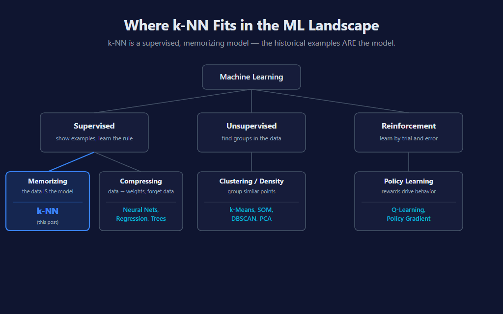
Within supervised learning there’s a deeper split most ML courses don’t make explicit but that matters enormously for trading: memorizing models vs. compressing models. Decision trees and k-NN memorize — the historical examples are literally the model. Neural networks and regression compress — they fit weights to the data, then throw the data away and predict using only those weights.
🧩 Why k-NN Is a Natural Fit for Charting Platforms
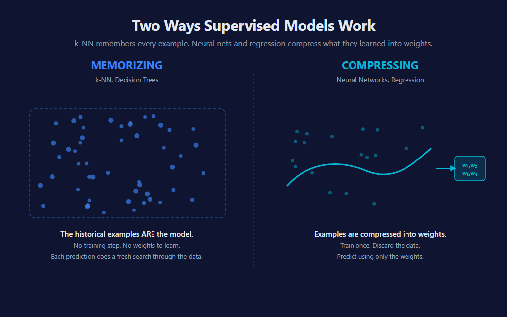
Charting platforms — Pine on TradingView, NinjaScript here in NT8 — share a structural constraint that shapes which ML approaches fit comfortably. A script lives inside the chart’s data feed and runs bar-by-bar; there’s no separate training step where you’d fit a model offline, persist weights, and load them back at runtime. Memorizing models like k-NN fit that constraint cleanly: the historical data is already on the chart, no weights to fit, no GPU required. Compressing models like neural networks need a training loop and somewhere to store the learned weights between runs — workable in a desktop ML stack, more friction inside a script that just sees bars.
That’s the practical reason k-NN shows up as the engine behind so many community-built ML indicators across charting platforms. It’s not a slight against the work — k-NN is genuinely one of the better fits for the environment, and a well-tuned k-NN can produce useful signals. The ones that work share a few traits we’ll cover later in the post: a small, well-chosen feature set; honest walk-forward validation; and gates that filter out the noisy predictions instead of trusting every search result.
🔑 The Three Concepts That Matter
Whether you write your own k-NN or evaluate someone else’s, three decisions drive everything: which features describe a bar, how distance between two bars is measured, and how many neighbors to poll. Get any of the three wrong and the model is (mostly) useless — but understanding all three is enough to read the majority of “AI” indicators on the market.
Features — what makes two bars similar
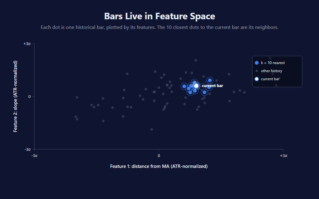
A “feature” is any number computed from a bar that captures something about its character. Distance from a moving average, the slope of recent prices, the bar’s volatility regime, RSI, body-to-range ratio — all features. The combination of features defines what “similar” means. Two bars with identical price but very different volatility regimes are not similar in a vol-aware feature space, but they would be in a price-only one.
Distance — how similarity gets measured
Once features are defined, every bar is a point in feature space. “Most similar” becomes the geometric problem of “closest by some distance metric” — usually Euclidean distance: sqrt((f1_today − f1_then)² + (f2_today − f2_then)² + …). Other metrics exist (Mahalanobis, correlation distance, dynamic time warping) but Euclidean is the universal default and what this indicator uses.
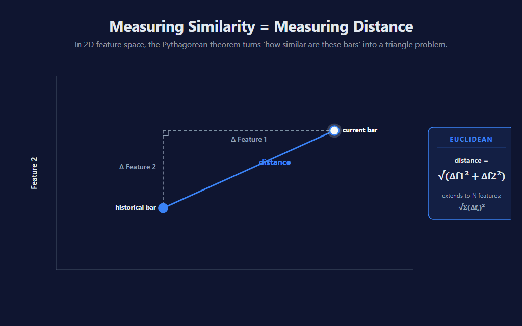
The visual makes the math literal: with two features, distance between any pair of bars is the hypotenuse of the right triangle whose legs are Δf1 and Δf2. The formula generalizes cleanly to any number of features — square each per-feature delta, sum, take the square root. That’s it. (For comparison-only purposes the indicator skips the square root and works in squared-distance space — same ordering, fewer ops.)
k — how many neighbors to ask
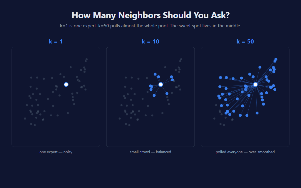
K=1 means take the single most-similar bar and use its outcome as the prediction. Noisy and overconfident — one outlier match and the prediction flips. K=50 means average across 50 matches. Smoother but the signal washes out toward the mean of the entire dataset. The sweet spot lives in the middle, and this indicator defaults to K=2 — favoring strong individual matches that haven’t been smeared out.
💪 What k-NN Does Well, and Where It Falls Short
k-NN’s strength is honesty. There’s nowhere for the model to hide. Every prediction comes with explicit historical analogs — you can pull the K matches up and look at them. No “the network has decided” mystery; the answer is literally “these are the bars that look like today, and this is what happened after them.” That property alone makes k-NN ideal for trading: you’re not betting on a black box, you’re betting on a database lookup.
The weakness is what’s called the curse of dimensionality. As you add more features, every bar in feature space drifts toward equidistant from every other bar — the volume of that space grows exponentially with dimensions while the historical data does not, so points spread out faster than samples can fill them. With a handful of features, “nearest” still means something concrete. By the time you’ve stacked a dozen or more, the gap between the closest and farthest neighbors compresses to the point where “nearest” starts to feel a lot like “average.”
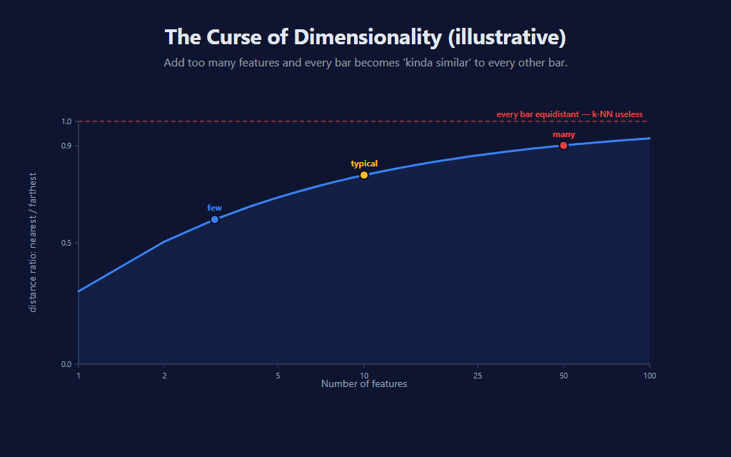
Practical takeaway: k-NN tends to work best with a small, well-chosen feature set. Adding features past that point usually hurts more than it helps — even when each new feature looks individually informative — because the distance signal in the K-nearest search degrades faster than the new information can compensate.
🛠️ Building the Indicator — Setup
Enough theory — let’s look at the actual indicator running. Default settings on NQ 1-minute show a mix of long and short signals across both trend continuation and turning points, each labeled with the predicted move and direction:
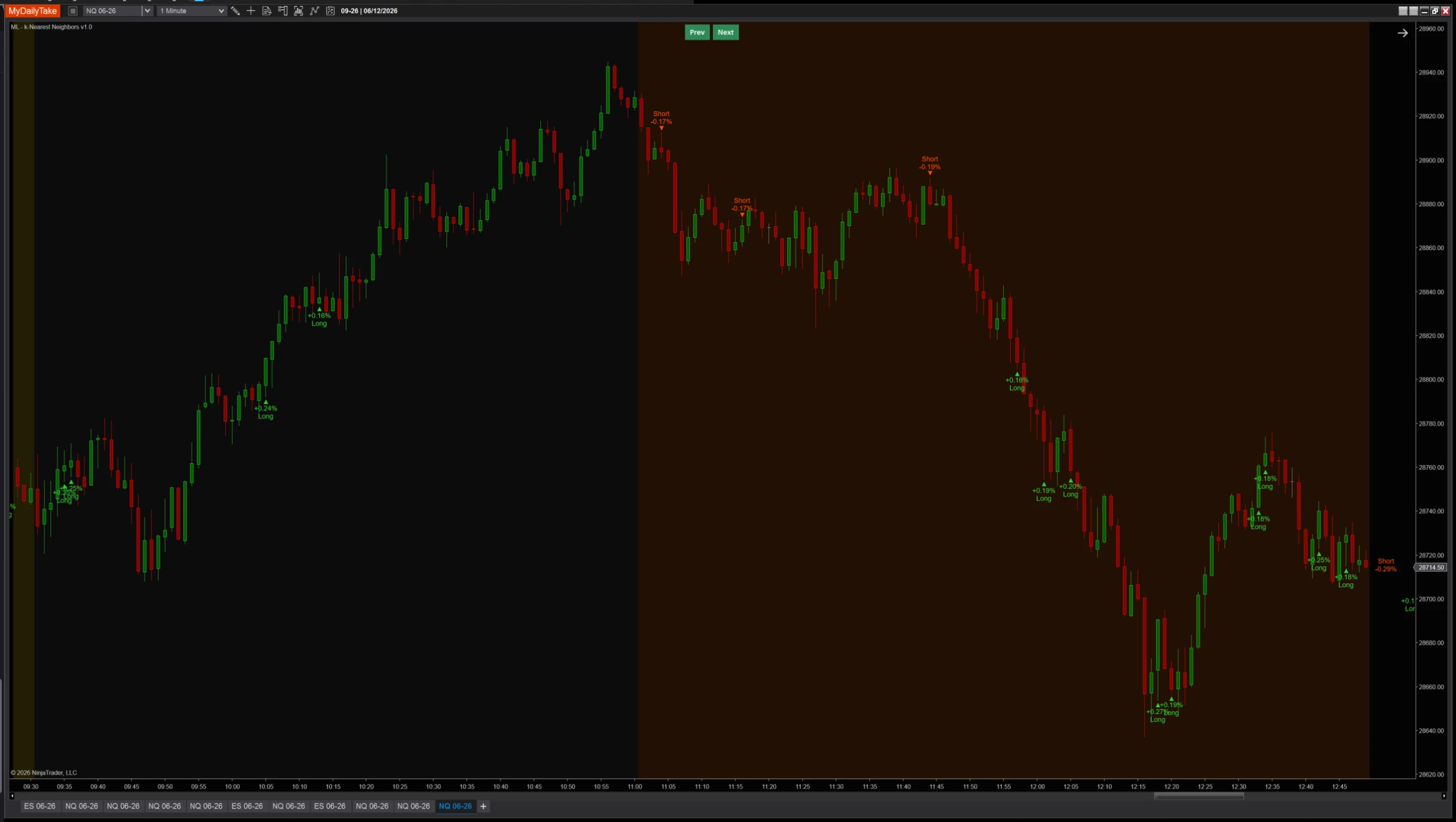
The indicator is a chart overlay only — no sub-panel. Each signal renders as a colored triangle next to the bar, plus a two-line label: predicted return % on the line nearest the triangle, direction word (Long / Short) on the other line. The label offset is configurable so you can dial in the spacing for your bar size.
🎯 The Features (Pure Trend-Following)
Three features, all ATR-normalized so the scale stays consistent across volatility regimes:
- distFromMa —
(Close − SMA(MaPeriod)) / ATR. How far above or below the moving average the bar is, expressed in volatility units. Captures directional position. - slope —
(Close − Close[SlopeLookback]) / ATR. How much price has moved over the slope window, in volatility units. Captures momentum thrust. - atrRegime —
ATR / SMA(ATR, MaPeriod). Current volatility relative to its own recent average — separates calm regimes from chaotic ones, so the model only matches against bars from similar regimes.
The implementation is intentionally compact — three numbers, written into a caller-supplied buffer so we never allocate inside the search hot loop:
private void GetFeaturesInto(double[] dst, int barsAgo)
{
    double atrVal	= atr[barsAgo];
    double safeAtr	= atrVal > 1e-9 ? atrVal : TickSize;

    // Distance from MA, in ATRs — directional position scaled by volatility.
    dst[0] = (Close[barsAgo] - trendMa[barsAgo]) / safeAtr;

    // N-bar slope, in ATRs — recent momentum thrust, normalized.
    int slopeBack = barsAgo + SlopeLookback;
    dst[1] = slopeBack <= CurrentBar
        ? (Close[barsAgo] - Close[slopeBack]) / safeAtr
        : 0;

    // Volatility regime — current ATR vs typical ATR.
    double atrSmaVal = atrRegimeMa[barsAgo];
    dst[2] = atrSmaVal > 1e-9 ? atrVal / atrSmaVal : 1.0;
}
A few non-obvious choices worth flagging. safeAtr guards against division-by-zero on the rare bar where ATR comes out to literally zero — falling back to TickSize means the feature degrades gracefully instead of producing NaN and corrupting downstream comparisons. The slope falls back to zero when SlopeLookback bars don’t yet exist behind the candidate (very early in history), which keeps the feature defined without poisoning the distance calculation. And every feature is divided by safeAtr so the units cancel — distance comparisons across volatility regimes stay meaningful instead of being dominated by whichever era had the largest raw price moves.
⚖️ Normalization — Regime-Relative, Not Global
Z-score normalization rescales each feature against a rolling mean and standard deviation so a “1-σ extreme reading” means the same thing across very different market environments. Without it, distance comparisons get dominated by whichever regime had the largest raw values — a 2008 bar with explosive volatility looks “more extreme” on every feature than a calm 2024 bar, no matter what the bar’s actual character was relative to its peers.
The non-obvious choice in this indicator is which rolling stats each candidate is normalized against. Each historical candidate is z-scored using its own local-time stats — the rolling mean and std-dev computed over the bars that came before that candidate, not the bars that came before today. A 2008 bar is judged against the 2008 distribution it actually lived in; a 2024 bar against 2024’s. Markets aren’t stationary, so feeding every candidate through today’s lens silently breaks the comparison.
private void NormalizeInto(double[] dst, double[] raw, int barsAgo)
{
    if (!NormalizeFeatures)
    {
        for (int k = 0; k < NumFeatures; k++) dst[k] = raw[k];
        return;
    }

    for (int k = 0; k < NumFeatures; k++)
    {
        // [barsAgo] — not [0] — uses each candidate's OWN local-time stats.
        // SMA / StdDev maintain rolling values at every historical bar, so
        // featureMean[k][barsAgo] is the mean computed over the
        // NormalizationLookback bars BEFORE that historical bar.
        double mean = featureMean[k][barsAgo];
        double std  = featureStd[k][barsAgo];
        dst[k] = std > 1e-9 ? (raw[k] - mean) / std : (raw[k] - mean);
    }
}
The crucial line is double mean = featureMean[k][barsAgo];. NT’s SMA(featureSeries, NormalizationLookback) maintains the rolling mean at every historical bar in O(1) per access — the rolling-window stats are already there waiting to be read at any historical index. Reading [barsAgo] gives that candidate’s local-time mean; reading [0] would give today’s. The same applies to featureStd[k][barsAgo]. With the per-candidate version a “1-σ reading” is regime-relative and meaningfully comparable across eras — that’s what makes the K-nearest search return matches that are actually similar in their own context.
🔍 The Search Loop — Don’t Cheat the Past
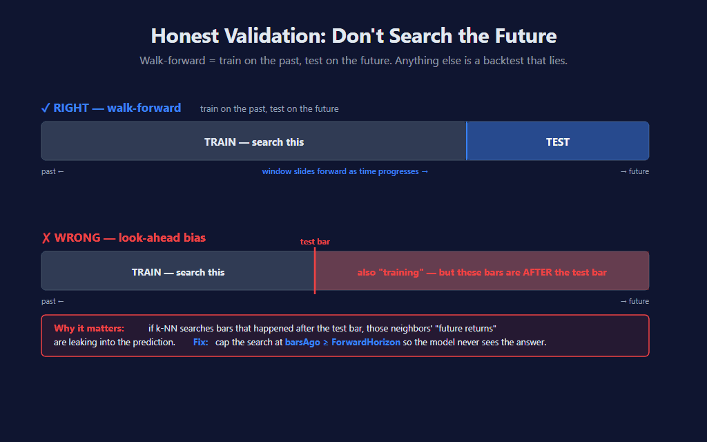
The search itself is straightforward: walk back through SearchLookbackBars bars, compute distance from today’s feature vector to each candidate’s, keep the K closest. Where it gets subtle is the look-ahead-prevention discipline.
Two invariants are enforced in the search loop:
barsAgo >= ForwardHorizon— every candidate must be at least N bars in the past, otherwise its “forward return” would peek into the future relative to that candidate.barsAgo <= CurrentBar − SlopeLookback— the slope feature itself needsSlopeLookbackbars before the candidate, otherwise the slope falls back to zero and contaminates the distance.
Both are hard caps, not soft suggestions. NinjaTrader’s bar-by-bar update model helps here — by the time OnBarUpdate fires for the current bar, all earlier bars are finalized data. We’re not constructing an artificial test set; the architecture itself prevents look-ahead as long as we respect the two invariants above.
// 1) Normalize the current bar against ITS own local-time stats.
NormalizeInto(currentNormBuf, scratchRaw, 0);

// 2) Cap the search window so look-ahead is impossible:
//    - lower bound: barsAgo >= ForwardHorizon  (forward returns must be observed)
//    - upper bound: barsAgo <= CurrentBar - SlopeLookback  (slope feature needs
//      Close[barsAgo + SlopeLookback], which has to exist)
int maxBarsAgo = Math.Min(SearchLookbackBars,
    Math.Min(CurrentBar - ForwardHorizon, CurrentBar - SlopeLookback));

int kBest = Math.Max(1, KNeighbors);
for (int i = 0; i < kBest; i++) bestDist[i] = double.MaxValue;
int filled = 0;

// 3) Walk back through history. For each candidate compute its features,
//    normalize using ITS local-time stats, measure squared distance to today,
//    and look up the realized forward return.
for (int barsAgo = ForwardHorizon; barsAgo <= maxBarsAgo; barsAgo++)
{
    GetFeaturesInto(scratchRaw, barsAgo);
    NormalizeInto(candidateNormBuf, scratchRaw, barsAgo);

    double dist = SquaredDistance(currentNormBuf, candidateNormBuf);

    double closeNeighbor = Close[barsAgo];
    double closeFuture   = Close[barsAgo - ForwardHorizon];
    double fwdReturn     = (closeFuture - closeNeighbor) / closeNeighbor;

    InsertTopK(bestDist, bestFwd, bestBarsAgo, ref filled, kBest, dist, fwdReturn, barsAgo);
}
The hot loop runs once per bar at signal time. maxBarsAgo compresses both look-ahead caps into a single bound the loop body never has to recheck. scratchRaw, currentNormBuf, candidateNormBuf, and the three best… arrays are all pre-allocated fields — no allocations inside the loop, even though we’re computing fresh feature vectors and comparing them thousands of times per bar. SquaredDistance deliberately doesn’t take the square root: we only need to order distances to find the K closest, and ordering is preserved by squaring. InsertTopK maintains the top-K in a single pass — no full sort.
📊 The Prediction & Two-Gate Signal
For each candidate match, the indicator records the realized forward return that occurred ForwardHorizon bars after that historical bar — i.e., what would have happened if you had taken the trade then. Across the K matches we compute the mean (the prediction) and the standard deviation (the spread / disagreement among matches).
A signal fires only when both gates pass:
- Magnitude gate —
|mean| > MinPredictedReturn. The predicted move has to be material. Default 0.0015 (15 bps over the forward horizon). - SNR gate —
|mean| / stddev > MinSignalToNoise. The K matches have to roughly agree. Default 0.3 — generous on purpose, since K=2 by default produces small samples.
The label on the chart shows the predicted mean forward return — i.e., the model’s “we think this bar will move X% over the next 30 bars.” That’s the model’s best estimate, not a guarantee. Backtest for yourself before trusting it.
// Aggregate across the K nearest neighbors:
//   prediction = mean forward return
//   confidence = std-dev of those returns
double sum = 0, sumSq = 0;
for (int i = 0; i < filled; i++)
{
    sum   += bestFwd[i];
    sumSq += bestFwd[i] * bestFwd[i];
}
double prediction = sum / filled;
double variance   = (sumSq / filled) - (prediction * prediction);
double std        = variance > 0 ? Math.Sqrt(variance) : 0;

// Two-gate signal qualification — both must pass for a triangle to fire:
//   - Magnitude gate: rejects tiny moves that aren't worth trading
//   - SNR gate: rejects coin-flip neighbor splits where matches disagree
double absPrediction = Math.Abs(prediction);
double snr           = std > 1e-12 ? absPrediction / std : double.PositiveInfinity;

bool meetsMagnitude  = absPrediction >= MinPredictedReturn;
bool meetsSnr        = snr >= MinSignalToNoise;
if (!(meetsMagnitude && meetsSnr)) return;
The std-dev calculation uses the single-pass identity variance = E[x²] − (E[x])² so we don’t need a second loop over the K neighbors. The two bool gates are deliberately combined with && — both must pass before any plot fires. With K=2 by default, the SNR gate is the more common rejector: two matches that disagree wildly produce a high std-dev relative to the mean and the trade is silently filtered. Tune MinPredictedReturn to control which moves are “big enough to bother with” and MinSignalToNoise to control how much neighbor disagreement you’ll tolerate.
📝 The Honest Validation Talk
An accuracy headline like “85%” by itself is hard to evaluate. The figure is meaningful only when it ships with two things alongside: the methodology used to compute it, and the test window it covers. Walk-forward validation (train on the past, test on the future, no overlap between the two) is the standard for non-stationary financial data — anything else lets information from the future leak into the model’s predictions and inflates the apparent accuracy. Whenever you see a quoted accuracy number, the question to ask is how it was measured. If that part isn’t shown, the number can’t be checked.
The harder problem is regime drift. Markets change — what worked from 2010 to 2018 may not work from 2020 forward. Even with perfect walk-forward methodology, a k-NN trained on the last 2000 bars is implicitly assuming the next bar lives in roughly the same regime as that window. When regimes shift (as they always eventually do), expect the edge to compress until the search window slides far enough forward to absorb the new regime. This is one reason the indicator’s SearchLookbackBars is configurable — shorter windows track regime changes faster but have less data to pattern-match against.
⚙️ Settings
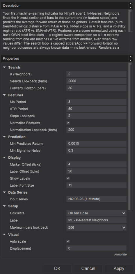
The indicator’s settings are grouped into four categories so the parameters that actually move the model live separately from the cosmetic ones.
Search
| Parameter | Description |
|---|---|
| K Neighbors | Number of historical bars to average for each prediction. K=1 is the single most-similar bar (noisy). K=50 dilutes the signal toward the global average. Default 2 — favors strong individual matches. |
| Search Lookback Bars | How far back the engine searches for similar bars. Larger windows give more candidates but also more regime drift. Default 2000. |
| Forward Horizon | How many bars ahead the historical 'forward return' is measured over. Also enforces a hard look-ahead barrier — candidates must be at least this many bars in the past. Default 30. |
Features
| Parameter | Description |
|---|---|
| MA Period | Lookback for the moving average used in the distFromMa feature. Smaller = more sensitive to short-term position; larger = trend-anchored. Default 8. |
| ATR Period | Lookback for the ATR used to normalize all three features. Default 50. |
| Slope Lookback | Number of bars over which the slope feature is measured (Close[0] − Close[N], ATR-normalized). Smaller = momentum thrust; larger = trend persistence. Default 2. |
| Normalize Features | Master toggle for z-score normalization. When ON, each feature is rescaled against its own historical rolling stats — letting the engine compare regimes fairly. Recommended ON. |
| Normalization Lookback | Window used to compute the rolling mean / stddev that z-score the features. Each candidate uses ITS OWN local-time stats (not today's). Default 200. |
Prediction
| Parameter | Description |
|---|---|
| Min Predicted Return | Magnitude gate. The mean forward return across the K neighbors must exceed this absolute value before a signal fires. Default 0.0015 (15 bps over the forward horizon). |
| Min Signal to Noise | Noise gate. |mean| / stddev across the K neighbors must exceed this ratio. Filters out predictions where the K matches disagree wildly. Default 0.3. |
Display
| Parameter | Description |
|---|---|
| Marker Offset (ticks) | Vertical offset of the triangle markers from the bar's high (shorts) or low (longs), in ticks. Default 4. |
| Label Offset (ticks) | Distance from the bar to the text label, in ticks. Should be larger than Marker Offset so the label sits beyond the triangle. Default 20. |
| Show Labels | Render the predicted-return % and direction label beside each marker. Turn off for a marker-only chart. |
| Label Font Size | Font size for the signal labels. Default 12. |
🎚️ Pairing With a Regime Filter
The indicator deliberately fires both with and against the prevailing trend — it’s a similarity model, not a trend follower, so the same setup can be a continuation buy in one regime and a counter-trend reversal attempt in another. Pairing it with a simple regime filter cleans that up immediately. RSI(14) above/below 50 is the simplest version: take longs only in the uptrend regime, shorts only in the downtrend regime, ignore the rest.
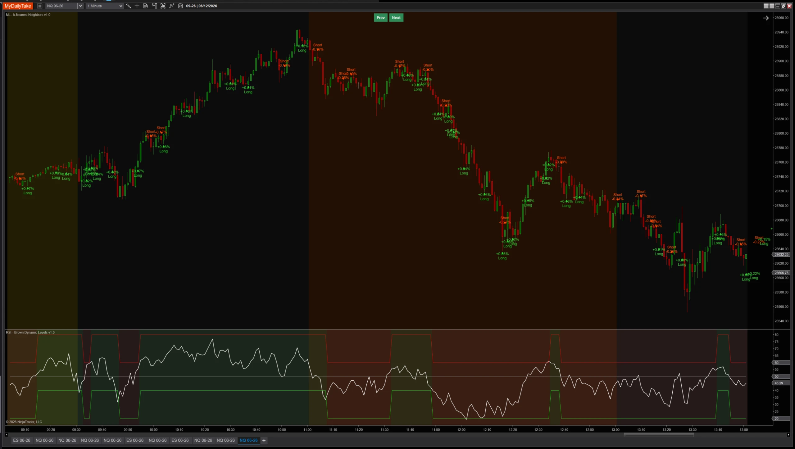
RSI is just the example — the same mental model fits any regime tool you already trust. ADX above a threshold, price relative to a higher-timeframe MA, a SuperTrend state, your own bias indicator. The point isn’t which filter you use; it’s that the k-NN signal and the regime call are two independent pieces of evidence, and both should agree before you take a trade.
🛠️ Using It in a Strategy
The indicator exposes every state it computes as a public Series so any NinjaScript strategy can reference it directly — no copy/paste of internals, no recomputation. The two signal Series (IsLongSignalSeries, IsShortSignalSeries) are the bool triggers; PredictionSeries and ConfidenceSeries let you size or filter further on the actual predicted magnitude and neighbor agreement.
Public Outputs
| Output | Type | Purpose |
|---|---|---|
| PredictionSeries |
Series | Mean forward return across the K nearest neighbors. The model's raw prediction. |
| ConfidenceSeries |
Series | Std-dev of the K neighbors' forward returns — lower = more agreement among matches. |
| NeighborAvgFwdReturnSeries |
Series | Alias of PredictionSeries, kept for naming clarity in chained strategies. |
| IsLongSignalSeries |
Series | True on bars where prediction passes both gates AND is positive. |
| IsShortSignalSeries |
Series | True on bars where prediction passes both gates AND is negative. |
To reference the indicator in a strategy: declare a private field of type MlKNearestNeighbors, initialize it in State.DataLoaded with whatever parameter set you want to back-test, then read knn.IsLongSignalSeries[0] (and friends) inside OnBarUpdate. Below, the same RSI regime filter shown above, wired up as a working strategy:
private MlKNearestNeighbors	knn;
private RSI					rsi;

protected override void OnStateChange()
{
    if (State == State.SetDefaults)
    {
        Name		= "KnnRsiTrendFollower";
        Calculate	= Calculate.OnBarClose;
    }
    else if (State == State.DataLoaded)
    {
        knn = MlKNearestNeighbors(
            kNeighbors:               2,
            searchLookbackBars:       2000,
            forwardHorizon:           30,
            maPeriod:                 8,
            atrPeriod:                50,
            slopeLookback:            2,
            normalizeFeatures:        true,
            normalizationLookback:    200,
            minPredictedReturn:       0.0015,
            minSignalToNoise:         0.3);

        rsi = RSI(14, 3);
    }
}

protected override void OnBarUpdate()
{
    if (CurrentBar < 250) return;

    // Long: model predicts up AND RSI confirms uptrend regime
    if (knn.IsLongSignalSeries[0] && rsi[0] > 50)
        EnterLong("k-NN Long");

    // Short: model predicts down AND RSI confirms downtrend regime
    if (knn.IsShortSignalSeries[0] && rsi[0] < 50)
        EnterShort("k-NN Short");
}
The pattern generalizes beyond RSI. Swap the filter for any indicator that exposes a Series — pair the k-NN signal with whatever regime evidence you already have on your charts. Multiple filters can be ANDed together for stricter setups, or used as separate trade-class strategies that each take a different slice of the model’s output.
📦 Download
Install:
- Download the .zip file above.
- In NinjaTrader 8, go to Tools → Import → NinjaScript Add-On.
- Select the downloaded .zip file.
- The indicator will appear under Indicators → indMyDailyTake → ML — k-Nearest Neighbors v1.0 on your chart.


This is the first installment of a Learn NinjaScript ML series — next up is online learning, the natural extension of k-NN that updates predictions as new bars arrive instead of treating every prediction as a fresh search. The MlKNearestNeighbors indicator is open source and released under MPL 2.0; modify, fork, and ship your own variants freely.
