
ML — Random Forest: An Ensemble of Decision Trees for NinjaTrader 8
Posts 2 through 7 of this series were one long thread. A single neuron became hidden layers, hidden layers became configurable depth, depth got a better optimizer, and then the network grew a memory and finally gated memory. Every one of those models learned the same way: compute a gradient, nudge the weights.
This post changes the model entirely. A Random Forest has no weights and no gradient — there is nothing to nudge. It is an ensemble of decision trees, each one a chain of simple yes/no questions on the features. Training a tree means building a structure, not tuning numbers. And the “forest” part — many trees, each grown on slightly different data — is what turns a fragile single tree into a genuinely useful model. This is the first of two posts on tree ensembles; the next covers gradient boosting.
🌳 Anatomy of a Decision Tree
A decision tree carves the feature space into boxes. Each internal node asks one question — is one feature at or below some threshold? — and routes the bar left or right. Follow the questions down and you land at a leaf, which stores a single number: the probability of an up move.
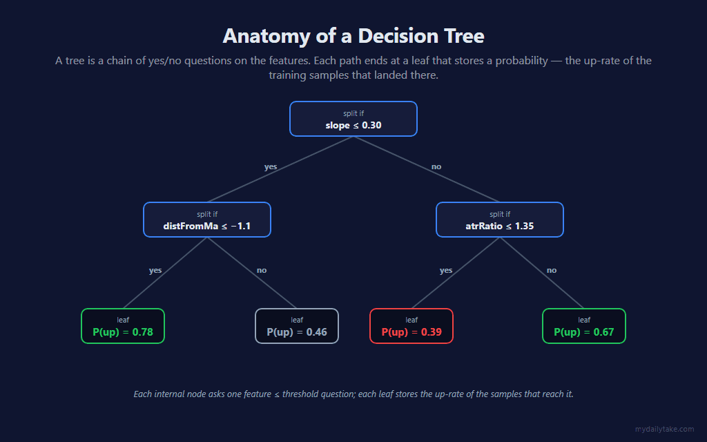
That leaf probability is not a guess — it is the empirical up-rate of the training samples that landed in that leaf’s box. If 78 of the 100 training bars that reached a leaf went on to close higher, the leaf’s P(up) is 0.78. The whole tree is a piecewise-constant function: every point in the feature space falls in exactly one leaf box and gets that box’s probability.
🪓 Choosing a Split — Gini Impurity
The cleverness of a tree is in where the cuts go. A good split makes its two child boxes purer — closer to all-up or all-down. The purity measure is Gini impurity. For a node with positive fraction p:
G = 2p(1 − p)
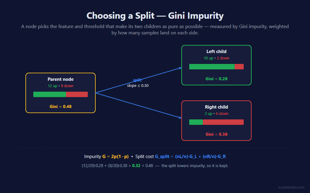
Gini is zero for a pure node and peaks at 0.5 for a pure coin-flip. A split sends some samples left and some right; its cost is the sample-weighted average of the two children’s impurity, G_split = (n_L/n)·G_L + (n_R/n)·G_R. The node tries every candidate threshold and keeps the split with the lowest G_split — but only if it actually beats the parent’s impurity. The candidate thresholds are the midpoints between consecutive sorted feature values; a sweep up the sorted list scores each one:
// Score every candidate split for a random subset of FeaturesPerSplit features
// and return the one that minimizes the Gini impurity of the two children.
// A split is kept only if it beats the parent's impurity and leaves at least
// MinSamplesLeaf samples on each side.

private bool FindBestSplit(int lo, int hi, int n, int totalPos, out int bestFeat, out double bestThr)
{
    bestFeat = -1;
    bestThr  = 0.0;

    double bestWeighted = Gini(totalPos, n);   // a split must improve on the parent
    bool   found        = false;

    ShuffleFeatureBag();

    for (int fi = 0; fi < FeaturesPerSplit; fi++)
    {
        int f = featureBag[fi];

        // sort this node's samples by feature f
        for (int s = 0; s < n; s++)
        {
            int ex = bootstrapIdx[lo + s];
            sortScratch[s].Value = trainFeat[ex][f];
            sortScratch[s].Label = trainLabel[ex];
        }
        Array.Sort(sortScratch, 0, n);

        // sweep a threshold between every pair of distinct values
        int leftPos = 0;
        for (int i = 0; i < n - 1; i++)
        {
            leftPos += sortScratch[i].Label;
            int leftN = i + 1;

            if (sortScratch[i].Value == sortScratch[i + 1].Value) continue;
            if (leftN < MinSamplesLeaf || (n - leftN) < MinSamplesLeaf) continue;

            int rightN   = n - leftN;
            int rightPos = totalPos - leftPos;
            double weighted = (leftN * Gini(leftPos, leftN) + rightN * Gini(rightPos, rightN)) / n;

            if (weighted < bestWeighted)
            {
                bestWeighted = weighted;
                bestFeat     = f;
                bestThr      = 0.5 * (sortScratch[i].Value + sortScratch[i + 1].Value);
                found        = true;
            }
        }
    }

    return found;
}

// Rearrange bootstrapIdx[lo..hi) so samples with feature[feat] <= thr come
// first; the returned index is the start of the right child.

private int Partition(int lo, int hi, int feat, double thr)
{
    int mid = lo;
    for (int s = lo; s < hi; s++)
    {
        if (trainFeat[bootstrapIdx[s]][feat] <= thr)
        {
            int tmp = bootstrapIdx[mid];
            bootstrapIdx[mid] = bootstrapIdx[s];
            bootstrapIdx[s]   = tmp;
            mid++;
        }
    }
    return mid;
}

// Gini impurity of a node with `pos` up-labels out of `n`:  G = 2p(1 - p).
private static double Gini(int pos, int n)
{
    double p = (double)pos / n;
    return 2.0 * p * (1.0 - p);
}
One detail worth noticing: the search only considers FeaturesPerSplit features, chosen at random, not all three. That restriction is deliberate, and the bagging section below explains why it matters.
🌲 Growing the Tree
Growing a tree is just that split, applied recursively. A node finds its best split, partitions its samples into two children, and each child repeats the process. The recursion stops — and the node becomes a leaf — at the depth cap, when the node is too small to split, when it is already pure, or when no split improves on its impurity:
// Grow one node of a tree. bootstrapIdx[lo..hi) are the sample slots for this
// node; the node is split in place and the two children are grown recursively.
// A node becomes a leaf at the depth cap, when it is too small to split, when
// it is already pure, or when no split improves on its impurity.

private int BuildNode(int treeIdx, int lo, int hi, int depth)
{
    RfNode[] tree = trees[treeIdx];
    int nodeIdx   = treeNodeCount[treeIdx]++;
    int n         = hi - lo;

    int pos = 0;
    for (int s = lo; s < hi; s++) pos += trainLabel[bootstrapIdx[s]];

    bool makeLeaf = depth >= MaxDepth || n < 2 * MinSamplesLeaf || pos == 0 || pos == n;

    int    bestFeat = -1;
    double bestThr  = 0.0;
    int    mid      = lo;
    if (!makeLeaf && FindBestSplit(lo, hi, n, pos, out bestFeat, out bestThr))
    {
        mid = Partition(lo, hi, bestFeat, bestThr);
        if (mid <= lo || mid >= hi) bestFeat = -1;   // degenerate split — make a leaf
    }

    if (makeLeaf || bestFeat < 0)
    {
        tree[nodeIdx].Feature  = -1;                 // -1 marks a leaf
        tree[nodeIdx].LeafProb = (double)pos / n;    // the leaf's P(up)
        return nodeIdx;
    }

    int left  = BuildNode(treeIdx, lo,  mid, depth + 1);
    int right = BuildNode(treeIdx, mid, hi,  depth + 1);

    tree[nodeIdx].Feature   = bestFeat;
    tree[nodeIdx].Threshold = bestThr;
    tree[nodeIdx].Left      = left;
    tree[nodeIdx].Right     = right;
    return nodeIdx;
}
This is a greedy procedure: each node takes the locally best cut and never reconsiders. The tree it produces is not the globally optimal tree — finding that is intractable — but greedy growth is fast, and the ensemble around it makes up for the greediness. Max Tree Depth and Min Samples per Leaf are the two knobs that bound how far a tree can carve before it starts fitting noise.
🎒 Bagging — Many Trees, Different Data
A single deep tree is a poor model on its own — it fits its training sample closely, so a slightly different sample produces a very different tree. It has low bias but high variance. The fix is not a better tree; it is many trees, averaged.
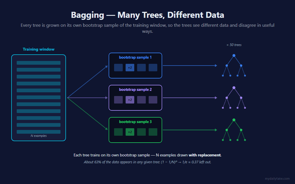
Every tree is grown on its own bootstrap sample: N examples drawn from the training window with replacement, where N is the size of the window. Drawing with replacement means some examples appear several times and others not at all — the probability an example is missed is (1 − 1/N)ᴺ, which approaches 1/e, so each tree sees roughly 63% of the data. Different data, different trees:
// Rebuild the whole forest. Each tree draws its own bootstrap sample — N
// indices drawn WITH replacement, where N is the number of training examples
// — then grows a decision tree on it. Called every RetrainInterval bars.

private void RebuildForest()
{
    int n = trainCount;
    for (int t = 0; t < NumTrees; t++)
    {
        for (int s = 0; s < n; s++)
            bootstrapIdx[s] = rng.Next(n);

        treeNodeCount[t] = 0;
        BuildNode(t, 0, n, 0);
    }
}
Averaging the predictions of many trees is called bagging (bootstrap aggregating). The math behind why it works is worth stating precisely: for an ensemble of trees each with prediction variance σ² and pairwise correlation ρ, the variance of the average is ρσ² + (1−ρ)/B · σ². As the number of trees B grows, the second term vanishes — but the first does not. The variance floor is ρσ², set entirely by how correlated the trees are. More trees help only until you hit that floor; to push the floor down, you have to make the trees disagree.
🎲 Feature Subsampling
Bootstrap sampling alone is not enough to decorrelate the trees. If one feature is strongly predictive, every tree splits on it first, and the trees end up looking alike — ρ stays high. So each split is only allowed to consider a random subset of the features:
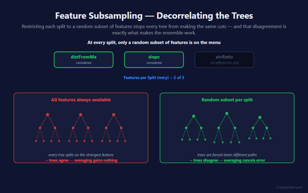
This is the “random” in Random Forest. Features per Split — the classic mtry parameter — defaults to 2 of the 3 features. It is a deliberate trade: each individual tree gets slightly weaker, because it is sometimes denied its best split, but the trees decorrelate, and ρ falls more than σ² rises. The ensemble comes out ahead. With only three features the effect is modest — there is not much room to subsample — but it is still the mechanism that makes the forest more than a pile of similar trees.
🗳️ The Forest Vote
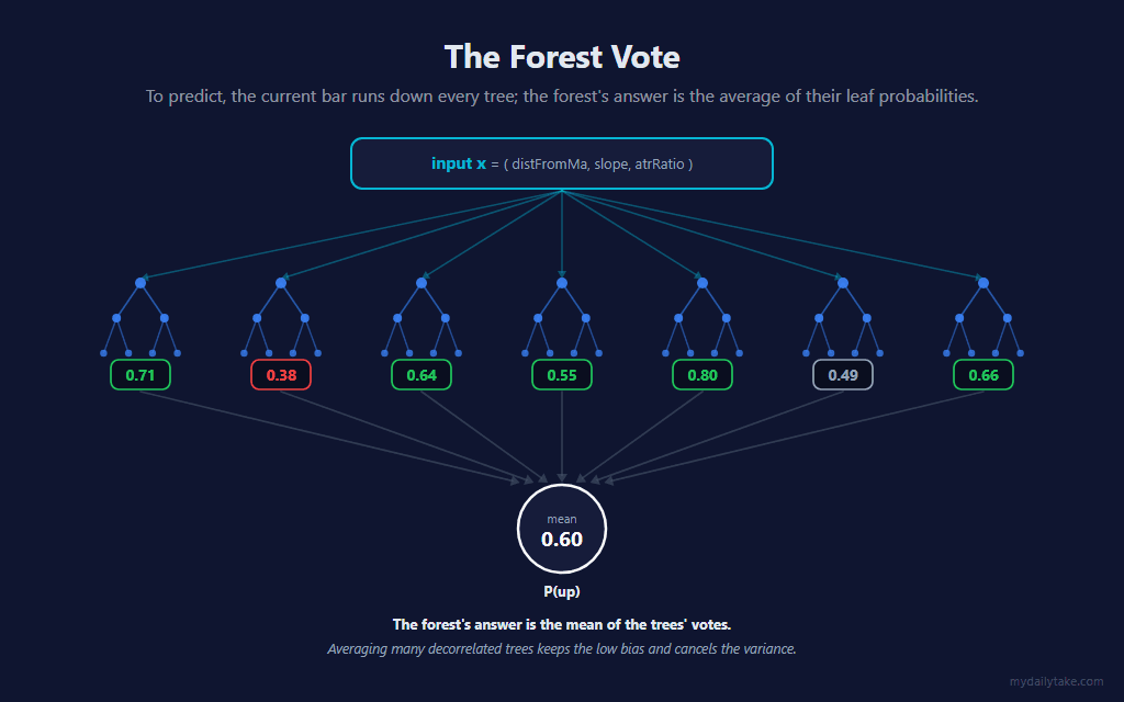
Prediction is the simplest part. The current bar’s feature vector runs down every tree; each tree lands in a leaf and returns that leaf’s probability. The forest’s answer is the plain average:
// The forest's prediction is the mean of the trees' votes.

private double ForestPredict(double[] feat)
{
    double sum = 0.0;
    for (int t = 0; t < NumTrees; t++) sum += PredictTree(t, feat);
    return sum / NumTrees;
}

// Walk one tree from the root: at each internal node go left if the feature is
// at or below the threshold, else right. The leaf's stored probability is the
// tree's vote.

private double PredictTree(int t, double[] feat)
{
    RfNode[] tree = trees[t];
    int idx = 0;
    while (tree[idx].Feature >= 0)
        idx = feat[tree[idx].Feature] <= tree[idx].Threshold ? tree[idx].Left : tree[idx].Right;
    return tree[idx].LeafProb;
}
Each tree on its own is a high-variance estimate. Averaging many decorrelated trees keeps their low bias and cancels much of the variance — the averaged surface is far smoother and steadier than any single tree’s piecewise-constant boxes.
🔄 Why the Forest Retrains in Batches
Here is the real structural break from the neural-net posts. Those models were online learners — every bar, one example nudged the weights a little. A Random Forest cannot work that way. A tree is a discrete structure of split decisions; one new example does not “nudge” a split, and incorporating it correctly could flip a threshold near the root, which changes every box beneath it. There is no cheap incremental update.
So the indicator retrains in batches. Every bar it appends one look-ahead-safe (features, label) example — the features from Label Horizon bars ago, paired with the now-observable realized direction — to a rolling buffer of the most recent Training Window examples. Every Retrain Interval bars, it throws the old forest away and builds a fresh one from that buffer. The model is therefore piecewise-constant in time: fixed between rebuilds, and stepping to a new forest at each retrain. The look-ahead-safety rule is unchanged from the rest of the series — every training example is fully resolved before it is used.
📊 What This Looks Like on a Chart
Same indicator, same NQ session. First, the default settings:
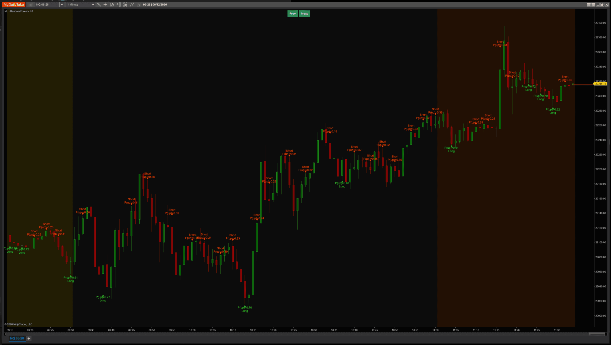
Default settings (Max Tree Depth = 6). The forest signals densely.
The first thing to notice is how often it fires. Compared with the gradient-trained models earlier in the series — which produced sparse clusters of signals — the forest is loud. That is not a bug, and it is worth understanding. A decision-tree leaf reports the empirical up-rate of its training box, which on real data is usually well away from 0.5; average fifty such votes and the result still lands away from 0.5 often enough to clear the Min Probability Edge gate frequently. The gradient-trained nets, by contrast, were pulled toward 0.5 by their regularizer. If the chart is too busy for you, raise Min Probability Edge or Signal Cooldown — those are the density knobs.
Now the depth comparison — shallow trees against deep ones:
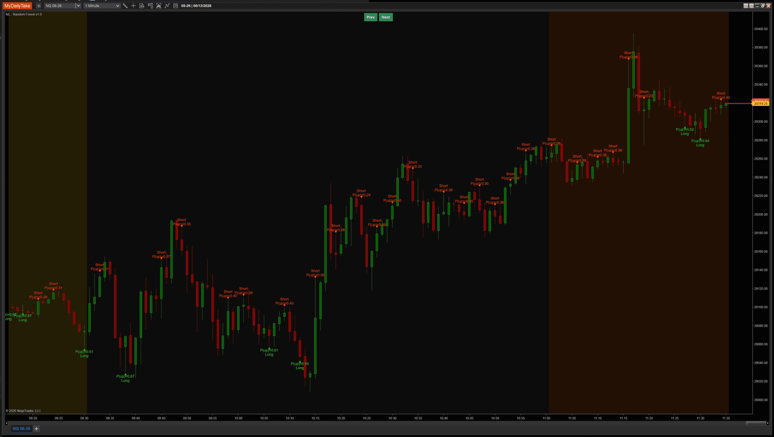
Max Tree Depth = 3 (shallow trees).
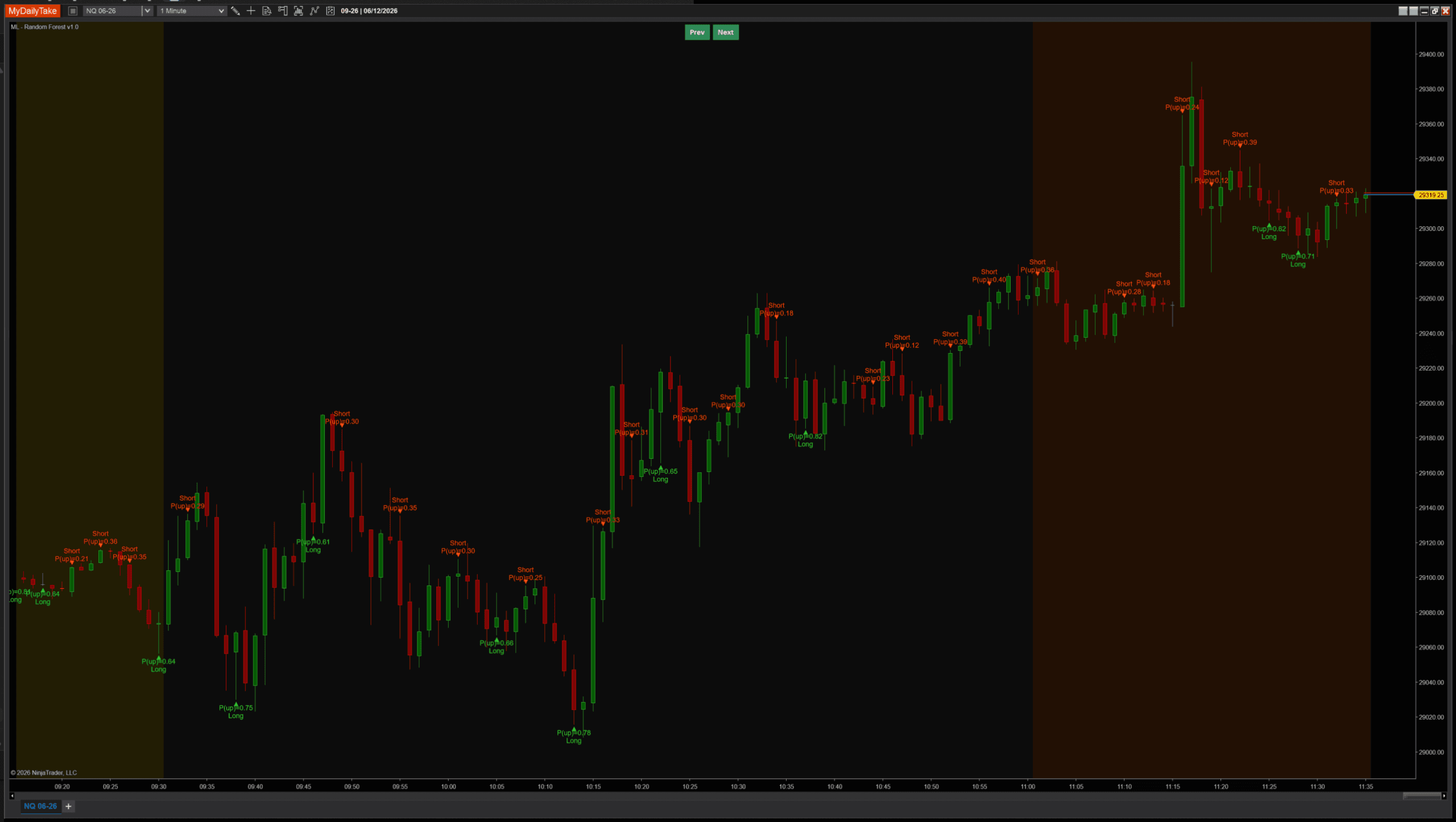
Max Tree Depth = 14 (deep trees).
Depth 3, 6, and 14 produce broadly similar charts — the exact probabilities and a handful of individual bars move, but the overall signal set does not transform. That is expected here, and it is reassuring rather than disappointing. Depth changes how finely each individual tree carves the feature space, but a fifty-tree ensemble averages most of that difference away, and with only three features there is not much fine structure for a deep tree to find that a shallow one misses. It is a small live demonstration of the standard Random Forest guidance: in a large ensemble, tree depth is a gentle knob, not a critical one.
⚙️ Settings
The indicator’s settings are grouped into five categories. Architecture sets the shape of the forest. Learning controls the training buffer, the retrain cadence, and the labeling. Features controls what the model sees. Signal controls when triangles fire. Display is cosmetic-only.
Architecture
| Parameter | Description |
|---|---|
| Number of Trees | Number of decision trees in the forest. Each tree is grown on its own bootstrap sample, and the forest prediction averages all of their votes. More trees = a smoother, lower-variance prediction but proportionally more compute on each retrain. Default 50. |
| Max Tree Depth | Maximum depth of each decision tree. Deeper trees can carve more detailed regions but are more prone to fitting noise. With only three features and noisy financial data, shallow trees in a large forest tend to generalize better. Default 6. |
| Min Samples per Leaf | Minimum number of training samples a node must keep on each side of a split. Larger values force bigger, more stable leaves and resist overfitting; smaller values let trees carve finer regions. Default 8. |
| Features per Split | Number of features (out of 3) randomly considered at each split — the 'mtry' of a Random Forest. Values below 3 decorrelate the trees, which is what makes the ensemble work. Default 2. |
| Random Seed | Seed for the bootstrap sampling and the per-split feature selection. The same seed and the same bar history produce the same forest — useful for reproducible testing. |
Learning
| Parameter | Description |
|---|---|
| Training Window (bars) | Number of recent look-ahead-safe (feature, label) examples kept for training. Each forest rebuild draws its bootstrap samples from this rolling window, so older examples fall out over time. Default 300. |
| Retrain Interval (bars) | How often the whole forest is rebuilt. A decision tree cannot be updated one bar at a time, so the model retrains in batches every N bars from the current Training Window. Smaller = more responsive but more compute. Default 25. |
| Label Horizon (bars) | How many bars ahead the realized direction is observed. Each bar contributes one training example using the features from N bars ago, whose forward outcome is now known — this keeps training look-ahead-safe. |
| Label Mode | How the training label is defined. CloseToClose: y = 1 if Close at the end of the Label Horizon window is above Close at the training bar. FavorableExcursion: y = 1 if the long-side favorable move beat the short-side move during the window (uses bar highs/lows); bars below Min Favorable Move are skipped as chop. |
| Min Favorable Move (ATRs) | ONLY USED WHEN Label Mode = FavorableExcursion. Minimum favorable excursion (in ATRs at entry) required during the post-bar window for the bar to become a training example. |
Features
| Parameter | Description |
|---|---|
| MA Period | Period of the moving average used in the distance-from-MA feature, and the smoothing window for the ATR regime-ratio feature. |
| ATR Period | Period of the ATR used to scale every feature into volatility units, so distance comparisons stay consistent across regimes. |
| Slope Lookback (bars) | Number of bars over which the slope feature is measured: (Close[0] − Close[N]) / ATR. |
| Normalize Features (Z-Score) | Master toggle for z-score normalization. Decision trees are scale-invariant to fixed transforms, but the rolling z-score still helps by making each feature stationary against its own recent distribution. Recommended ON for parity with the rest of the series. |
| Normalization Lookback (bars) | Window used to compute the rolling mean and standard deviation that z-score the features. Each bar uses its own local-time stats. |
Signal
| Parameter | Description |
|---|---|
| Min Probability Edge | How far the forest's predicted probability of an up move must be from 0.5 before a signal fires. 0.10 means a long fires when P(up) > 0.60 and a short fires when P(up) < 0.40. |
| Signal Cooldown (bars) | Minimum number of bars between consecutive signals. Higher values space signals out so the chart stays readable. |
Display
| Parameter | Description |
|---|---|
| Marker Offset (ticks) | Vertical offset of the signal triangle from the bar's high (shorts) or low (longs), in ticks. |
| Label Offset (ticks) | Distance from the bar to the text label, in ticks. Should be larger than Marker Offset so the label sits beyond the triangle. |
| Show Labels | Render the predicted-probability label beside each signal triangle. |
| Label Font Size | Font size for the signal labels. |
One note on Normalize Features: decision trees are invariant to any fixed monotonic rescaling of a feature — a split threshold just moves with it — so unlike the neural nets, a forest does not need normalization. The toggle is kept on for parity with the rest of the series, and because the rolling z-score is not a fixed transform: it re-centres each feature against its own recent distribution, which does help on non-stationary market data. It is a genuine choice here, not a requirement.
🎚️ Pairing With a Regime Filter
Same defensive pattern as the prior posts, and the dense signal set makes it more useful here, not less. An RSI(14) above or below 50 vetoes counter-trend signals, so the forest is only allowed to fire with the broader trend:
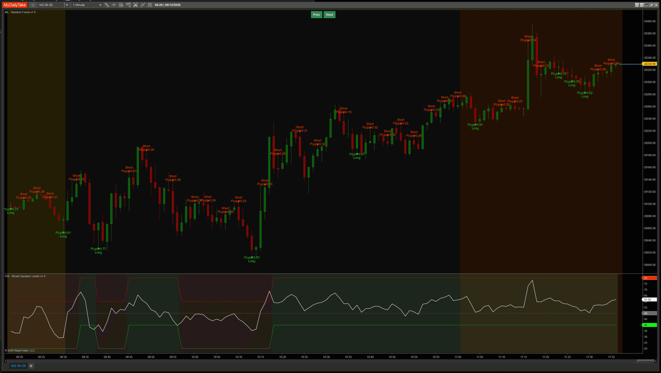
The forest’s raw output is a probability; the regime filter is a separate, far simpler model. Combining a learned signal with a transparent rule-based veto is a dependable way to keep the model from fighting the obvious trend.
🛠️ Using It in a Strategy
The indicator exposes its outputs as public Series so a strategy can consume the forest directly:
Public Outputs
| Output | Type | Purpose |
|---|---|---|
| ProbabilityUpSeries |
Series | The forest's predicted probability of an up move — the average of the trees' leaf probabilities. Range [0, 1]. |
| ConfidenceSeries |
Series | |P(up) − 0.5| × 2 — distance from a coin-flip, scaled to [0, 1]. 0 = uncertain, 1 = maximum conviction. |
| IsLongSignalSeries |
Series | True on bars where the prediction passes the probability gate AND the cooldown — a long signal fires. |
| IsShortSignalSeries |
Series | True on bars where the prediction passes the probability gate AND the cooldown — a short signal fires. |
Below is a working strategy that combines the forest’s signal with the RSI regime filter from the previous section — a long is allowed only when the forest predicts up and RSI is above 50, and the mirror for shorts:
private MlRandomForest      nn;
private RSI                 rsi;

protected override void OnStateChange()
{
    if (State == State.SetDefaults)
    {
        Name        = "RandomForestRsiTrendFollower";
        Calculate   = Calculate.OnBarClose;
    }
    else if (State == State.DataLoaded)
    {
        nn = MlRandomForest(
            numTrees:               50,
            maxDepth:               6,
            minSamplesLeaf:         8,
            featuresPerSplit:       2,
            randomSeed:             42,
            trainingWindow:         300,
            retrainInterval:        25,
            labelHorizon:           2,
            labelMode:              MlRandomForest_LabelMode.CloseToClose,
            minFavorableMoveAtrs:   1.0,
            maPeriod:               8,
            atrPeriod:              50,
            slopeLookback:          2,
            normalizeFeatures:      true,
            normalizationLookback:  200,
            minProbabilityEdge:     0.10,
            signalCooldownBars:     3);

        rsi = RSI(14, 3);
    }
}

protected override void OnBarUpdate()
{
    // The indicator gates its own signals through warmup; this is a safety margin.
    if (CurrentBar < 400) return;

    // Long: the forest predicts up AND RSI confirms the uptrend regime.
    if (nn.IsLongSignalSeries[0] && rsi[0] > 50)
        EnterLong("RF Long");

    // Short: the forest predicts down AND RSI confirms the downtrend regime.
    if (nn.IsShortSignalSeries[0] && rsi[0] < 50)
        EnterShort("RF Short");
}
📝 The Honest Validation Talk (Still)
A Random Forest is a strong, well-understood model — but a strong model on a hard problem is still constrained by the problem. Directional prediction from three features is close to a coin flip, and the forest’s dense, confident-looking signal stream can read as more certainty than the data supports. The model also has its own quiet trap: it retrains in batches, so its behavior steps from one forest to the next, and “accuracy over the last N bars” averages over several different forests. None of that is a reason to avoid it. It is a reason to evaluate it honestly — walk-forward across multiple regimes is still the only honest test, and the work scales with how seriously you intend to trust the result.
📦 Download
Install:
- Download the .zip file above.
- In NinjaTrader 8, go to Tools → Import → NinjaScript Add-On.
- Select the downloaded .zip file.
- The indicator will appear under Indicators → indMyDailyTake → ML – Random Forest v1.0 on your chart.


This is the eighth installment of the Learn NinjaScript ML series. Posts 1–7 built the neural-network thread — k-Nearest Neighbors, online logistic regression, a single hidden layer, configurable depth, the Adam optimizer, a recurrent network, and the LSTM. Post 8 (this one) leaves gradient descent behind for an ensemble of decision trees. Post 9 takes the tree idea further with gradient boosting.