ML — Online Logistic Regression: Your First Neural Net for NinjaTrader 8
The k-Nearest Neighbors post introduced one half of supervised learning: memorizing models that hold onto every historical bar and search through them at prediction time. This post is the other half. Instead of remembering every example, an online-learning model carries a small set of weights — three numbers, plus a bias term, in this case — and updates them one bar at a time as new data arrives. The historical data isn’t stored. The model itself is the compressed version.
Today we build that model in NinjaScript: online logistic regression, which is a fancy way of saying “a single neuron with a sigmoid that updates its weights every bar.” Calling it your first neural network is technically accurate — a single neuron is the simplest possible neural network. Once we wire one up and watch its weights evolve through a regime change, the path from here to a multi-neuron network (the next post in this series) is a one-step extension.
🧠 What “Online Learning” Actually Means
Most ML models you’ve seen are trained offline — fit on a fixed historical dataset, weights frozen, then deployed to make predictions. Online learning flips that: the model trains and predicts in the same loop, one example at a time. There’s no “training set” separate from “live use.” Every new bar is both an inference query (what’s P(up)?) and, eventually, a training example (here’s what actually happened — adjust the weights). The model never stops learning.
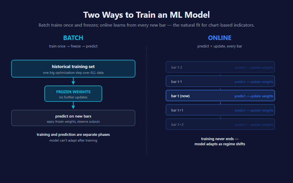
For chart-based indicators, online learning is the natural fit. The data already arrives bar-by-bar. There’s no separate training phase to schedule, no model file to load, no GPU to allocate. The state of the model lives in a few private fields on the indicator class, and they update inside OnBarUpdate like any other rolling calculation.
🌊 What a Single Neuron Actually Is
A neuron — in the technical, mathematical sense — is a function that takes some inputs, multiplies each by a weight, sums them, adds a bias term, and runs the result through an activation function. That’s it. There’s nothing biological about it; the “neuron” name is a 1950s analogy that stuck.
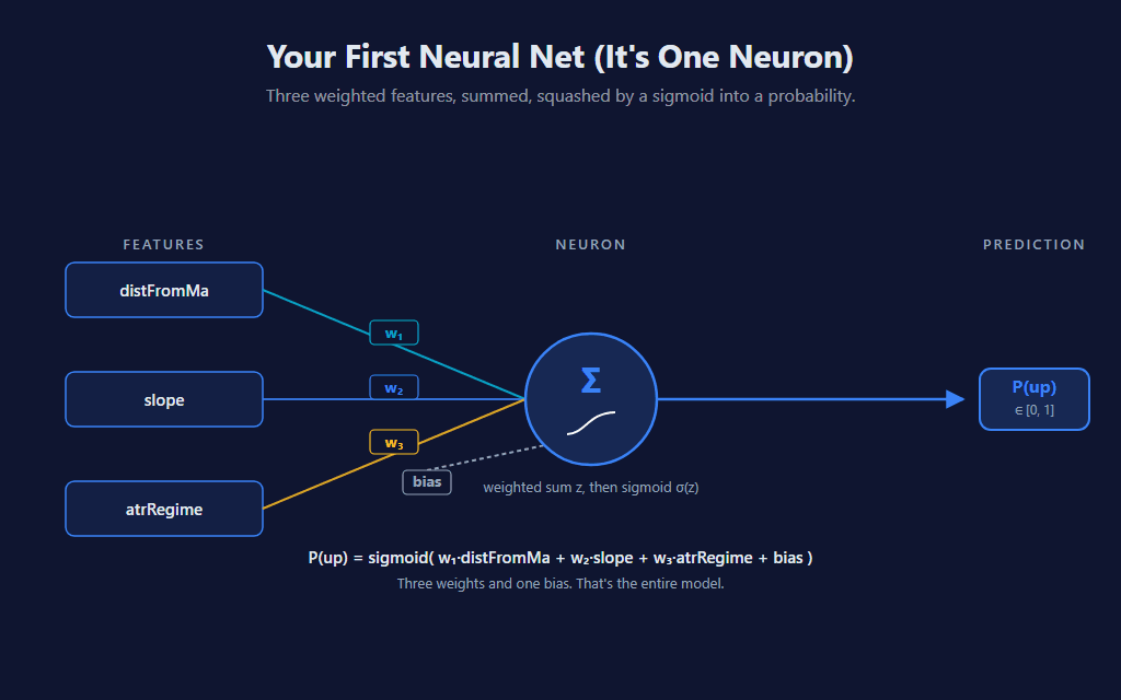
Our neuron has three inputs (the same three features as the k-NN sibling, kept identical so you can compare both indicators on the same chart), three weights, and a bias term. Total parameters: four numbers. The activation is a sigmoid, which gives us a probability output instead of an arbitrary real number. The math fits on a napkin:
P(up) = sigmoid( w₁·distFromMa + w₂·slope + w₃·atrRegime + bias )
📈 How a Number Becomes a Probability
The sigmoid (also called the logistic function — and yes, that’s where the name “logistic regression” comes from, even though it’s a classification algorithm) takes any real number and squashes it into the [0, 1] range. Large positive input → output near 1. Large negative input → output near 0. Zero input → exactly 0.5. The transition is smooth, and the derivative is mathematically convenient for gradient descent (which we’ll get to shortly).
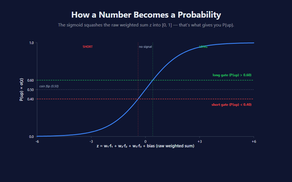
Once we have P(up), we apply two horizontal gates: signals only fire when the probability is meaningfully different from coin-flip. Default MinProbabilityEdge = 0.10 means long fires when P(up) > 0.60 and short fires when P(up) < 0.40. Anything between is treated as “no signal — model isn’t confident enough.”
🔁 The Online Loop: Predict → Wait → Compare → Adjust
Online learning isn’t really one algorithm — it’s a four-step loop that runs every bar. Predict using current weights. Wait until the forward outcome is observable. Compare the prediction to what actually happened. Adjust the weights so the prediction would have been more correct. Repeat. Forever.
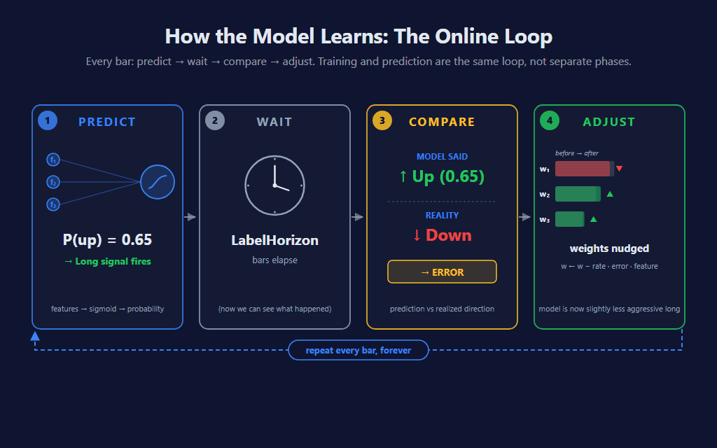
This is the architecture’s superpower: the model is always learning. It can never go stale because there’s no fixed training set to be stale against. When the regime shifts, the weights migrate to fit the new regime over the next several hundred bars. The cost is that the model also can’t anticipate a regime change before it happens — it can only learn from one that already started.
🎯 The Three Features (Same as k-NN)
To make this indicator directly comparable with the k-NN sibling on the same chart, we use the same three pure trend-following features:
- distFromMa —
(Close − SMA(MaPeriod)) / ATR. Directional position scaled by volatility. - slope —
(Close − Close[SlopeLookback]) / ATR. Recent momentum thrust, normalized. - atrRegime —
ATR / SMA(ATR, MaPeriod). Current volatility relative to recent average.
Each is z-score normalized using its own local-time stats, so a “1-σ extreme reading” means the same thing across regimes. (See the k-NN post for the full discussion of why local-time normalization matters more than the textbook ML default for non-stationary financial data.) The forward pass is then a single weighted sum followed by the sigmoid:
// Forward pass — runs every bar to compute P(up).
// Uses the CURRENT weights (the most recent post-training state).
NormalizeInto(scratchNorm, scratchRaw, 0);

double zCurrent = bias;
for (int k = 0; k < NumFeatures; k++)
    zCurrent += weights[k] * scratchNorm[k];

double pUp = Sigmoid(zCurrent);
scratchNorm holds the z-score-normalized features for the current bar; weights and bias are the model’s state, which evolves as we train. Sigmoid() is a static helper that handles input clamping to avoid overflow on extreme weighted sums. Three lines of math. That’s the whole prediction.
⚖️ Two Ways to Label a Bar
This is the indicator’s most consequential parameter — the one that fundamentally changes what the model learns. To train, we need a label y for each historical bar: a 1 if it should have been a long, a 0 if it should have been a short. There are two reasonable ways to define that label, and they produce dramatically different models on the same data.
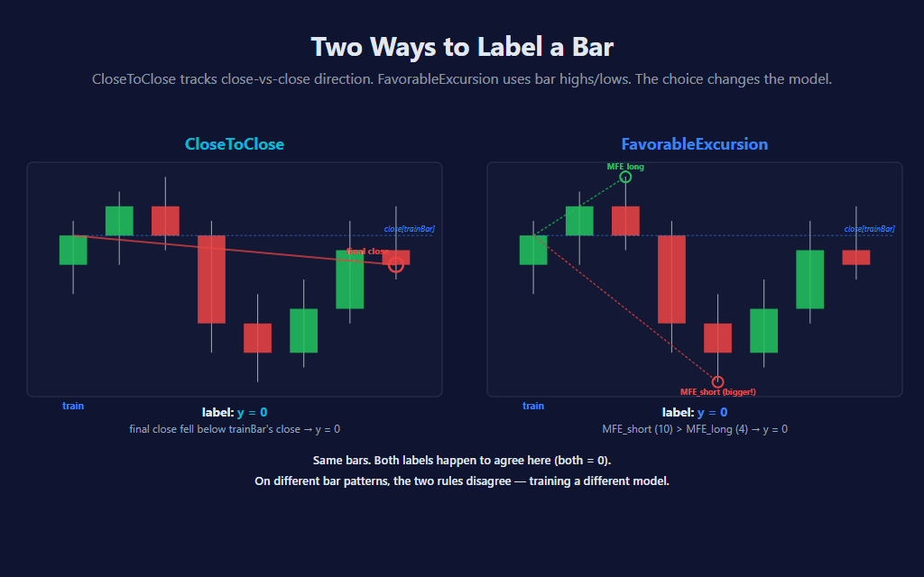
CloseToClose is the simplest. The label is just whether Close[0] ended up higher or lower than Close[trainBar] (LabelHorizon bars ago). Tracks pure close-to-close direction. Trains on every observable bar.
FavorableExcursion is more trader-aligned. It scans the bars between trainBar and now, finds the maximum favorable excursion in each direction (using bar highs for long excursion and lows for short), and asks: which side reached further? If neither side hit the MinFavorableMoveAtrs threshold, the bar’s follow-on was just chop and the model skips the update entirely — it doesn’t pretend there was a tradeable move where there wasn’t one. This is the more honest label for “would this have been tradeable?” but it’s also more sensitive to wicks.
// Two label modes — the choice fundamentally shapes the model's character.
//
//   CloseToClose:        y = direction of close-vs-close over LabelHorizon bars.
//                        Trains on every observable bar.
//
//   FavorableExcursion:  y = which side had the bigger MFE during the window
//                        (uses bar highs/lows). Skip when neither side hit
//                        Min Favorable Move — chop bars don't train.

bool   trainThisBar = false;
double y            = 0.0;

if (LabelMode == MlOnlineLogisticRegression_LabelMode.CloseToClose)
{
    y = Close[0] > Close[trainBar] ? 1.0 : 0.0;
    trainThisBar = true;
}
else // FavorableExcursion
{
    double closeAtTrain = Close[trainBar];
    double safeAtrTrain = atr[trainBar] > 1e-9 ? atr[trainBar] : TickSize;

    double maxHigh = double.MinValue;
    double minLow  = double.MaxValue;
    for (int b = 0; b < LabelHorizon; b++)
    {
        if (High[b] > maxHigh) maxHigh = High[b];
        if (Low[b]  < minLow)  minLow  = Low[b];
    }

    double mfeLong  = (maxHigh    - closeAtTrain) / safeAtrTrain;
    double mfeShort = (closeAtTrain - minLow)     / safeAtrTrain;

    if (Math.Max(mfeLong, mfeShort) >= MinFavorableMoveAtrs)
    {
        y = mfeLong > mfeShort ? 1.0 : 0.0;
        trainThisBar = true;
    }
}
Here’s where the choice gets real. The same indicator, on the same data, with the same features and the same weights — switching only LabelMode — produces different models. On a sustained uptrend day, FavorableExcursion at short horizons can produce too many short signals because intra-bar wicks down register as “short side won this bar.” CloseToClose ignores wicks and tracks pure direction. The chart below is the same trending day — left, FavorableExcursion; right, CloseToClose:
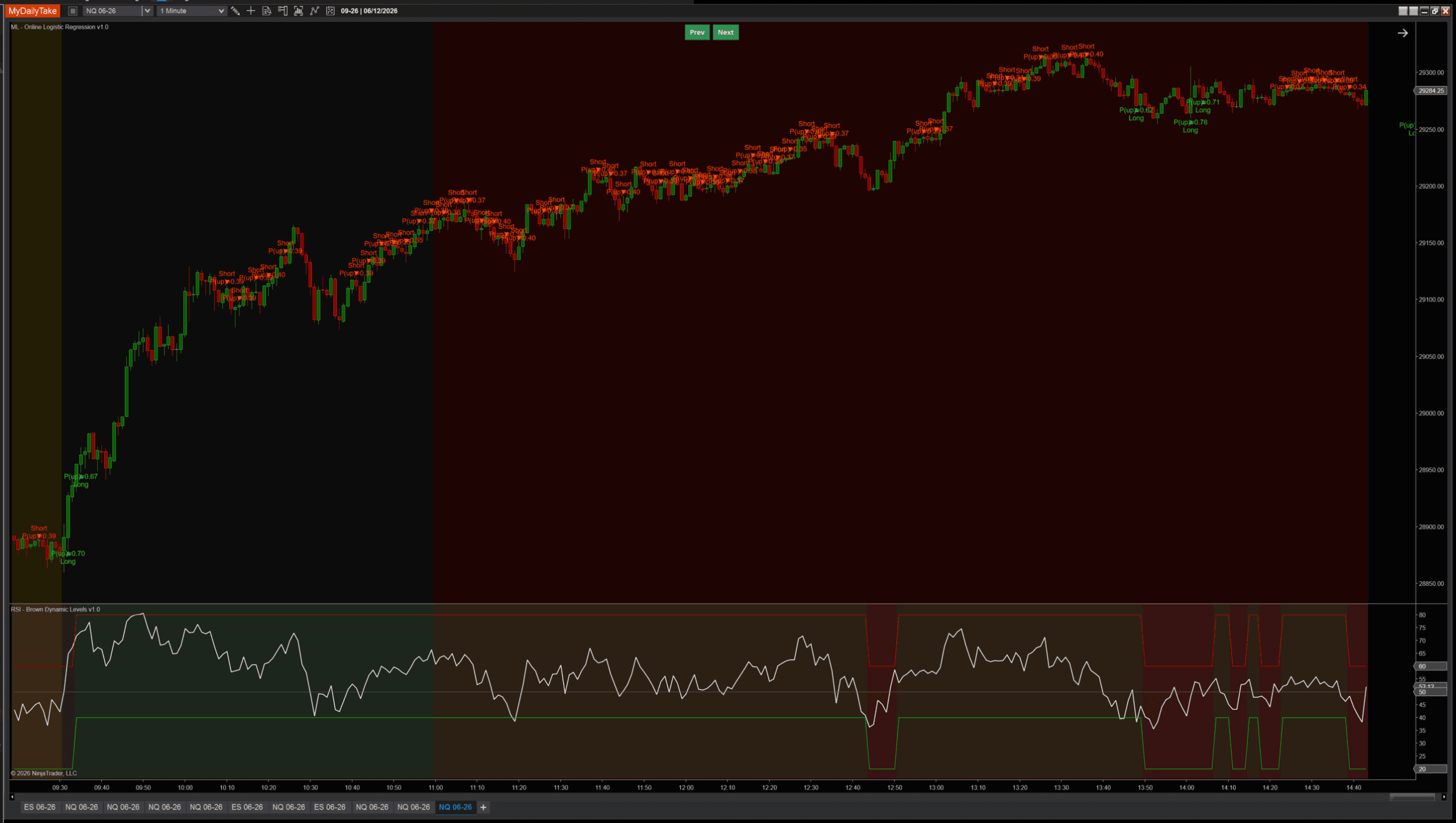
FavorableExcursion: too many shorts during a sustained uptrend.
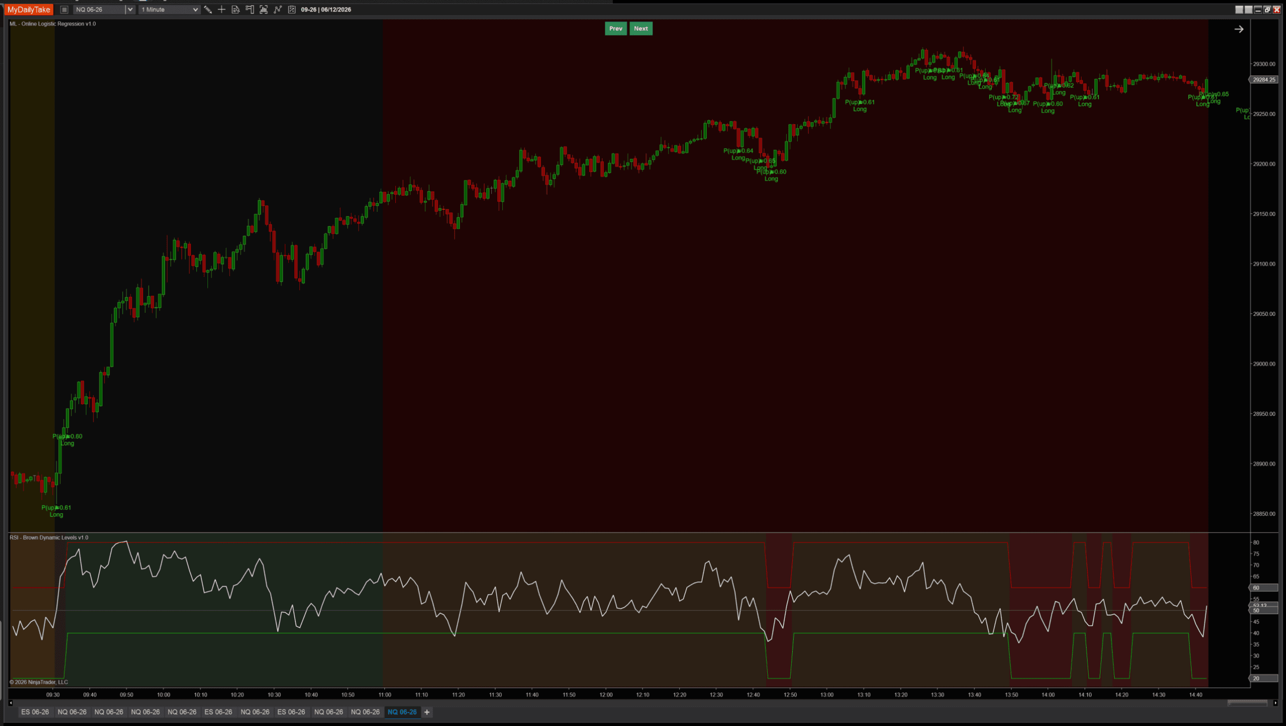
CloseToClose: clean trend-following on the same data.
Same indicator, same data, same features, same weights — switching only the label rule produces a different model. There’s no “right” answer — FavorableExcursion is better for catching tradeable opportunities in choppy data; CloseToClose is better for following sustained directional moves. The post ships with one as the default, but the parameter is one click away. The lesson worth keeping: the choice of label is arguably the most important parameter in any supervised ML model, far more than the learning rate or regularization. The label defines what the model is trying to predict.
📐 The Update Step (Gradient Descent in Plain English)
Once we have a label y and a prediction p, training is one step of gradient descent: nudge each weight a tiny amount in the direction that would have made the prediction more correct. The math comes from the cross-entropy loss function, but the formula is striking simple in code:
// Update step — runs every bar (when training conditions are met).
// Uses the bar from LabelHorizon ago, whose forward outcome is now observable.
GetFeaturesInto(scratchRaw, trainBar);
NormalizeInto(scratchNorm, scratchRaw, trainBar);

// Forward pass at trainBar with the CURRENT weights.
double zTrain = bias;
for (int k = 0; k < NumFeatures; k++)
    zTrain += weights[k] * scratchNorm[k];
double pTrain = Sigmoid(zTrain);

// Cross-entropy gradient: dL/dw_i = (p − y) · f_i, dL/db = (p − y).
// L2 regularization adds λ·w_i to each weight gradient (bias not regularized).
double error = pTrain - y;

for (int k = 0; k < NumFeatures; k++)
    weights[k] -= LearningRate * (error * scratchNorm[k] + RegularizationLambda * weights[k]);

bias -= LearningRate * error;
The error error = pTrain − y is positive when the model predicted higher than reality (over-confident long), negative when it predicted lower (over-confident short). Each weight gets nudged by −learning_rate × error × feature_value, which means: when the model was wrong, the weights connecting strongly-active features get adjusted the most. The L2 regularization term (λ·w) is a small additional pull toward zero on each step, keeping any single weight from running away on noisy bars.
The bias term updates the same way without the regularization (it represents the model’s class prior — its sense of how often things tend to go up vs down — and shouldn’t be artificially pulled toward zero).
📊 Watching the Model Adapt
The weights aren’t fixed. They start near zero (or small random values) and migrate over time as the model is exposed to data. During a single regime they settle into a stable band. When the regime changes, they migrate again — and the slope weight in particular can flip sign, going from “rising slope predicts up” to “rising slope predicts down” in a different market environment.
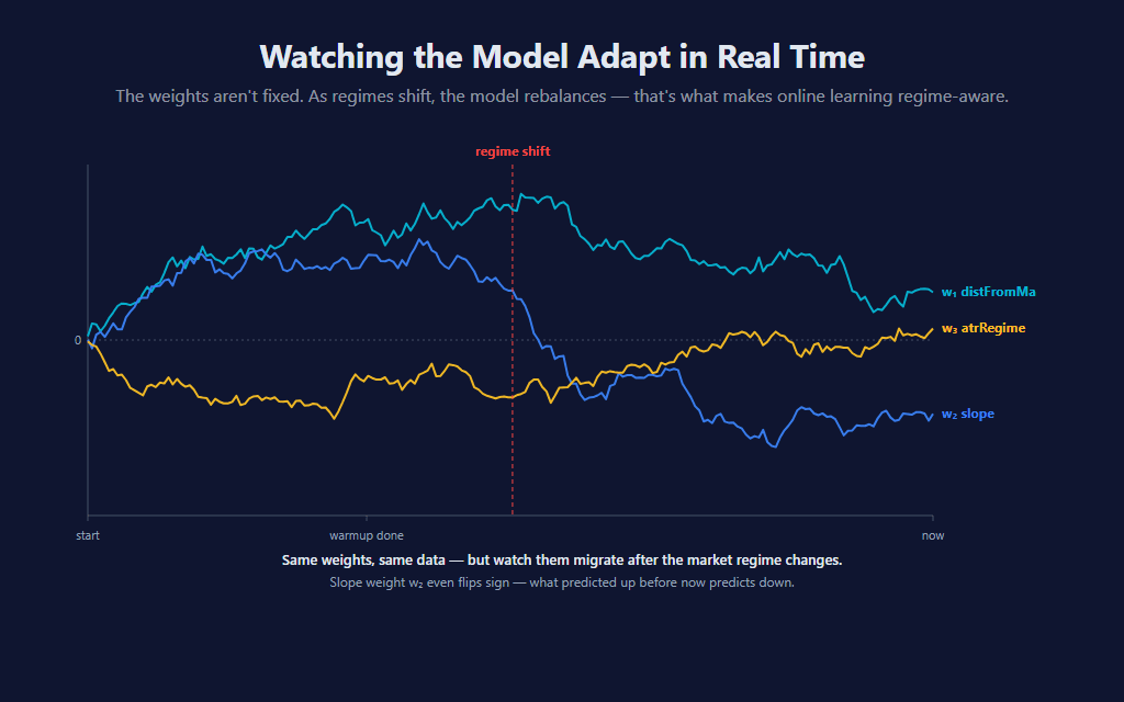
This is the architectural promise of online learning made literal: the model adapts. It doesn’t need to be retrained on a new dataset; the new dataset trains it as it arrives. The cost is that adaptation takes time — typically a few hundred update steps after a regime shift before the weights catch up.
💪 Where the Model Wins, and Where It Falls Apart
A single-neuron classifier is fundamentally a linear model in feature space. The decision boundary — the set of feature combinations where P(up) = 0.5 — is a hyperplane. Any pattern that requires non-linear interaction between features (e.g., “high distFromMa AND positive slope predicts continuation, but high distFromMa AND negative slope predicts reversal”) cannot be represented exactly. The next post in the series adds a hidden layer, which lets the model learn those interactions.
The other failure mode is more subtle: across a typical mix of regimes, bars with extreme distFromMa or slope often revert more than they continue, since most of the time markets aren’t sustaining a strong directional move. The model picks this tendency up, learns “extreme features tend to revert,” and produces good signals during normal market chop. But in a sustained directional trend — where every bar has extreme features and the trend keeps going — the same learned rule produces wrong-side counter-trend signals. The earlier two-chart comparison shows exactly this: FavorableExcursion’s spam of contrarian shorts during a clean uptrend.
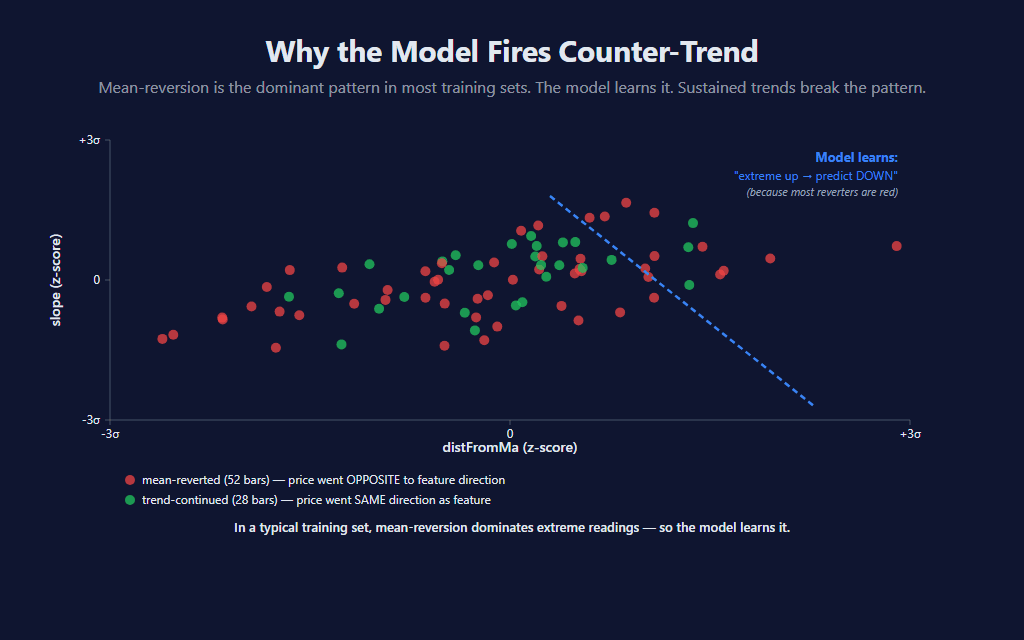
This isn’t a bug — it’s an architectural property. A single-neuron model trained on momentum-style features will always tend toward this behavior. There are several ways to mitigate it: pair the indicator with a regime filter (covered below), tune the learning rate higher to make the model adapt faster during regime shifts, or add features that capture trend persistence directly (multi-timeframe alignment, time-since-last-pullback, etc.). The proper fix is architectural — multiple neurons, hidden layers — and that’s the subject of post 3.
🛠️ Building the Indicator — Setup
Default settings on NQ 1-minute showing both directions firing across a typical mixed-regime session:
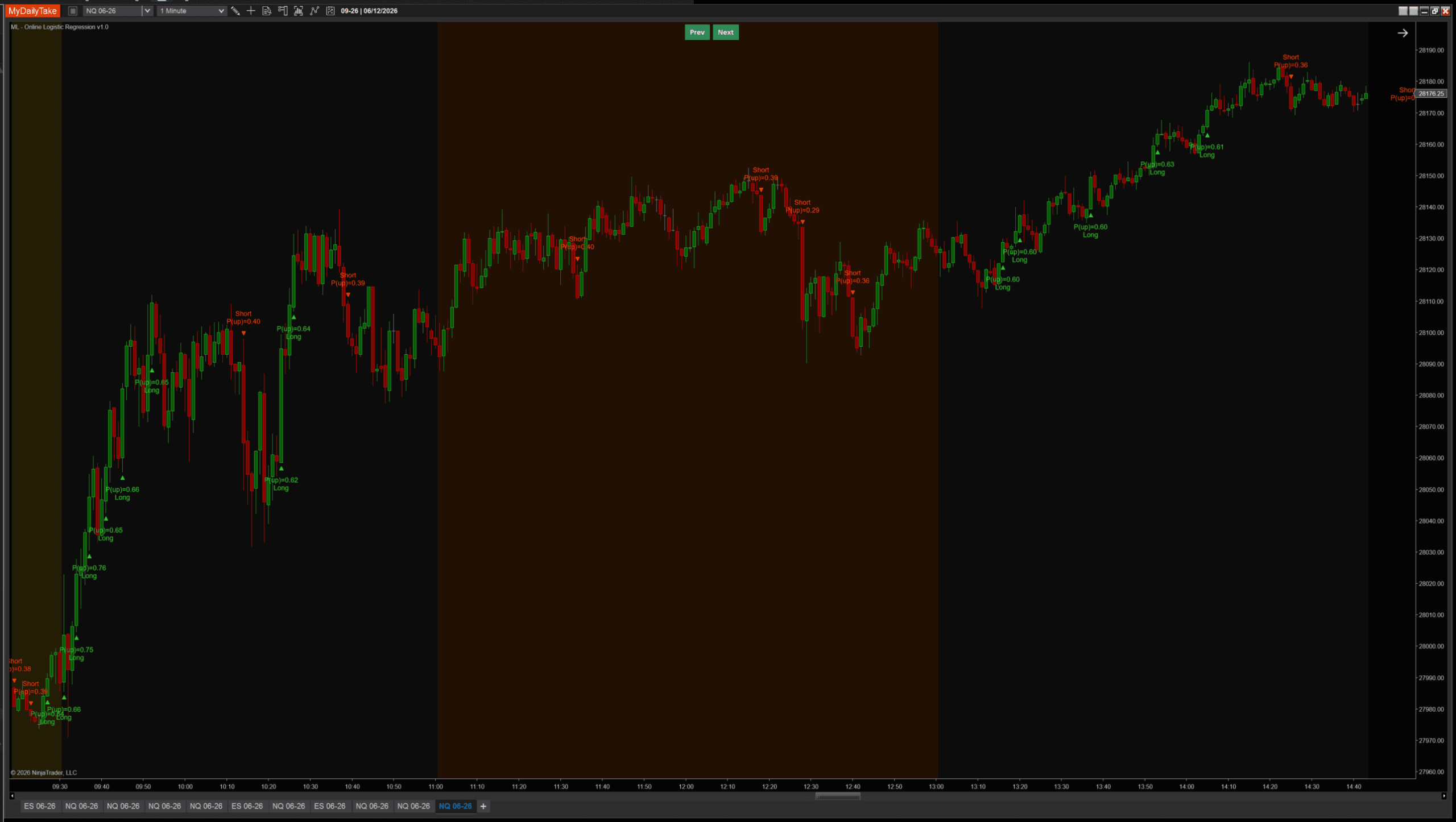
The indicator renders as a chart overlay — green TriangleUp markers below long-signal bars, red TriangleDown markers above shorts, plus a two-line label showing the predicted P(up) and direction. Same visual language as the k-NN sibling so they read consistently when both are on the same chart.
⚙️ Settings
The indicator’s settings are grouped into four categories. Learning controls how the model adapts; Features controls what the model sees; Signal controls when triangles fire; Display is cosmetic-only.
Learning
| Parameter | Description |
|---|---|
| Learning Rate | Step size for each weight update. Larger = adapts faster but jitters; smaller = smoother but slower to react. Practical sweet spot is 0.005 to 0.05 for normalized features. |
| Regularization Lambda (L2) | L2 penalty that pulls weights gently toward zero each update so they don't drift to extreme values when a feature is noisy. 0 disables regularization. |
| Label Horizon (bars) | How many bars ahead the realized direction is observed. The model updates each bar using the feature vector from N bars ago, whose forward direction is now known — this is what makes the training step look-ahead-safe. |
| Weight Init | Zero starts every weight at 0 (model takes longer to commit but has no built-in bias). Random starts with small random values around 0 (faster to commit; non-deterministic across reloads). |
| Label Mode | How the training label is defined. CloseToClose: y = 1 if Close at end of LabelHorizon window is above Close at trainBar. FavorableExcursion: y = 1 if max favorable excursion in the LONG direction beat the SHORT direction during the window — uses bar highs/lows so wicks count, and skips bars below Min Favorable Move (chop). The choice fundamentally shapes the model's character. |
| Min Favorable Move (ATRs) | ONLY USED WHEN Label Mode = FavorableExcursion. Minimum favorable excursion (in ATRs at entry) required during the post-bar window for the model to update. Below this threshold, the bar's follow-on was just chop — we skip the weight update. Set to 0 to train on every observable bar. |
Features
| Parameter | Description |
|---|---|
| MA Period | Period of the moving average used in the distFromMa feature, and used as the smoothing window for the ATR regime ratio. Smaller = more reactive; larger = trend-anchored. |
| ATR Period | Period of the ATR used to scale every feature into volatility units, so distance comparisons stay consistent across regimes. |
| Slope Lookback (bars) | Number of bars over which the slope feature is measured: (Close[0] − Close[N]) / ATR. Smaller = momentum thrust; larger = trend persistence. |
| Normalize Features (Z-Score) | Master toggle for z-score normalization. When ON, each feature is rescaled against its own historical rolling stats so a 1-σ extreme reading means the same thing across regimes. Recommended ON. |
| Normalization Lookback (bars) | Window used to compute the rolling mean / stddev that z-score the features. Each bar uses its own local-time stats — a 2008 bar against 2008's distribution, a 2024 bar against 2024's. |
Signal
| Parameter | Description |
|---|---|
| Min Probability Edge | How far the predicted probability of an up move must be from 0.5 before a signal fires. 0.10 means: long fires when P(up) > 0.60, short fires when P(up) < 0.40. Larger values produce fewer, higher-conviction signals. |
| Signal Cooldown (bars) | Minimum bars between consecutive signals. Higher values space signals out so the chart stays readable; lower values let signals come in clusters during sustained moves. Set to 0 to fire on every qualifying bar. |
Display
| Parameter | Description |
|---|---|
| Marker Offset (ticks) | Vertical offset of the signal triangle from the bar's high (shorts) / low (longs), in ticks. |
| Label Offset (ticks) | Distance from the bar to the text label, in ticks. Should be larger than Marker Offset so the label sits beyond the triangle. |
| Show Labels | Render the predicted-probability label beside each signal triangle. Turn off for a marker-only chart. |
| Label Font Size | Font size for the signal labels. |
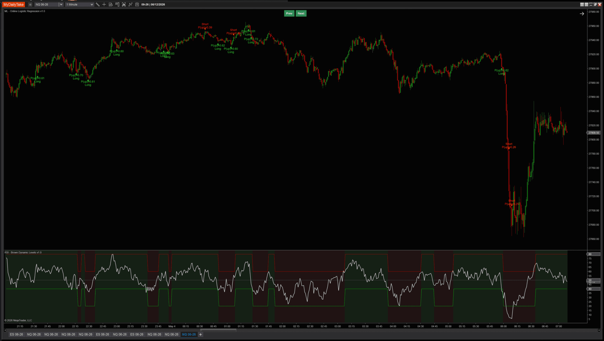
🎚️ Pairing With a Regime Filter
Because the model is biased toward mean-reversion at extremes, the cleanest practical use is to pair it with an external trend filter that vetoes counter-trend signals. RSI(14) above/below 50 is the simplest version: take longs only when RSI confirms uptrend regime, take shorts only when it confirms downtrend. The point isn’t which filter — ADX, higher-timeframe MA, your own bias indicator all work — but that the OLR signal and the regime call are independent pieces of evidence, and both should agree.
🛠️ Using It in a Strategy
The indicator exposes everything it computes as public Series, so any NinjaScript strategy can chain off it directly without recomputing the model. Probability, confidence, individual weight values, bias, and the boolean signal series are all available.
Public Outputs
| Output | Type | Purpose |
|---|---|---|
| ProbabilityUpSeries |
Series | The model's predicted probability of an up move, post-sigmoid. Range [0, 1]. |
| ConfidenceSeries |
Series | |P(up) − 0.5| × 2 — distance from coin-flip, scaled to [0, 1]. 0 = uncertain, 1 = maximum conviction. |
| WeightDistFromMaSeries |
Series | Current weight on the distFromMa feature. Positive = high distFromMa pushes prediction up. |
| WeightSlopeSeries |
Series | Current weight on the slope feature. Watch for sign flips during regime changes. |
| WeightAtrRegimeSeries |
Series | Current weight on the atrRegime feature. |
| BiasSeries |
Series | Current bias term — the model's default lean independent of features. |
| IsLongSignalSeries |
Series | True on bars where prediction passes the probability gate AND cooldown — long signal fires. |
| IsShortSignalSeries |
Series | True on bars where prediction passes the probability gate AND cooldown — short signal fires. |
Below: a working strategy that combines the model’s signal with an RSI regime filter. Long only when the model fires AND RSI confirms uptrend; short only when both confirm downtrend. The same pattern from the k-NN strategy example, with the OLR Series Plug-in:
private MlOnlineLogisticRegression	olr;
private RSI							rsi;

protected override void OnStateChange()
{
    if (State == State.SetDefaults)
    {
        Name		= "OlrRsiTrendFollower";
        Calculate	= Calculate.OnBarClose;
    }
    else if (State == State.DataLoaded)
    {
        olr = MlOnlineLogisticRegression(
            learningRate:           0.01,
            regularizationLambda:   0.0001,
            labelHorizon:           2,
            weightInit:             MlOnlineLogisticRegression_WeightInitMode.Zero,
            labelMode:              MlOnlineLogisticRegression_LabelMode.CloseToClose,
            minFavorableMoveAtrs:   1.0,
            maPeriod:               8,
            atrPeriod:              50,
            slopeLookback:          2,
            normalizeFeatures:      true,
            normalizationLookback:  200,
            minProbabilityEdge:     0.10,
            signalCooldownBars:     3);

        rsi = RSI(14, 3);
    }
}

protected override void OnBarUpdate()
{
    if (CurrentBar < 300) return;

    // Long: model predicts up AND RSI confirms uptrend regime
    if (olr.IsLongSignalSeries[0] && rsi[0] > 50)
        EnterLong("OLR Long");

    // Short: model predicts down AND RSI confirms downtrend regime
    if (olr.IsShortSignalSeries[0] && rsi[0] < 50)
        EnterShort("OLR Short");
}
Swap the RSI for any indicator that exposes a Series. ADX above a threshold, price relative to a higher-timeframe MA, a SuperTrend state — anything you already trust as a regime tool.
📝 The Honest Validation Talk
Online-learning models present a unique validation challenge: every prediction is technically out-of-sample (the bar being predicted hasn’t been used to update the weights yet — that happens LabelHorizon bars later), so traditional accuracy metrics work directly. But the model is also continuously changing, which means an “accuracy over the last 1000 bars” figure averages over many different effective models. The number you compute is more like a regime-weighted average than a stable model property.
If you see an accuracy headline for any ML indicator without methodology — what was the test window, what regime did it cover, was the model retrained or fixed — the number can’t be checked. Walk-forward across multiple regimes is the only honest way to evaluate this kind of model, and it takes substantially more work than a single chart screenshot can convey.
📦 Download
Install:
- Download the .zip file above.
- In NinjaTrader 8, go to Tools → Import → NinjaScript Add-On.
- Select the downloaded .zip file.
- The indicator will appear under Indicators → indMyDailyTake → ML — Online Logistic Regression v1.0 on your chart.
🎉 Prop Trading Discounts
💥89% off at Bulenox.com with the code MDT89
This is the second installment of the Learn NinjaScript ML series. Post 1 covered k-Nearest Neighbors, the memorizing model. Post 2 (this one) covered online logistic regression, the simplest compressing model. Post 3 will add a hidden layer — your first actual multi-layer neural network — and unlock the non-linear feature interactions that a single neuron can’t represent.


![Cosine Kernel Regressions [QuantraSystems] Conversion](https://mydailytake.com/wp-content/uploads/2024/06/CosineKernelRegressions_5-Minute_NQ-768x458.png)