ML — Long Short-Term Memory (LSTM): Gated Memory for NinjaTrader 8
The previous post built a vanilla Recurrent Neural Network — a model with a hidden state that carries forward bar to bar — and then ran straight into its defining limitation. Training a recurrent network means multiplying the gradient by a tanh derivative at every step back through time, and a long chain of numbers below one collapses toward zero. Ten steps back, the training signal reaching the oldest bars was roughly one part in a thousand. The vanilla RNN could learn short-range structure and almost nothing beyond it.
The Long Short-Term Memory network — the LSTM — was designed specifically to fix that. It keeps the recurrent idea but adds a second state, the cell state, plus three gates that control it. The cell state gives the gradient a path back through time that is not squashed at every step — and that one structural change is what lets an LSTM learn patterns that span far more bars than a vanilla RNN ever could.
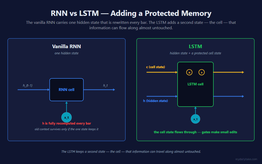
🧠 RNN vs LSTM — Adding a Protected Memory
A vanilla RNN carries exactly one state vector. Every bar, that hidden state is completely recomputed — old context survives only if the single state happens to keep encoding it. The LSTM splits memory into two:
- The hidden state
h— the working output. It still feeds the prediction and still flows into the next bar’s gates, exactly like the RNN’s hidden state. - The cell state
c— a separate memory vector that runs through the cell on its own track. Crucially, the gates only make small, controlled edits to it each bar — a little erased, a little written. Information can ride the cell state across many bars almost untouched.
That second state is the whole idea. The RNN had one channel that was rewritten wholesale every step; the LSTM adds a channel that is protected by design.
🔬 Inside the LSTM Cell
Internally, the cell is the cell-state “highway” plus four small gate networks that control it. Each gate reads the current bar’s features and the previous hidden state, and outputs a vector of valves:
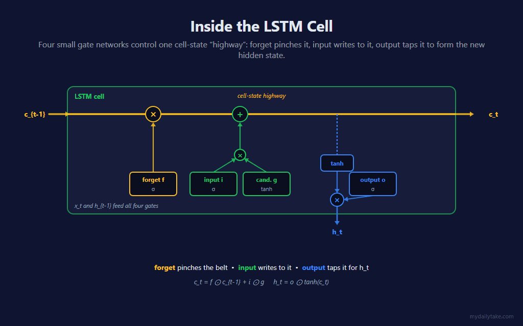
Reading the cell update left to right: the forget gate multiplies the incoming cell state — deciding what to keep and what to drop. The input gate and the candidate together decide what new information to add. The result is the new cell state. Then the output gate taps that cell state — through a tanh — to produce the new hidden state. In two lines:
c_t = f ⊙ c_{t-1} + i ⊙ gh_t = o ⊙ tanh(c_t)
The ⊙ is an element-wise product — each gate is a vector the same size as the cell, so every cell neuron gets its own keep/write/expose decision. Four gate networks instead of the RNN’s single recurrent matrix means the LSTM carries roughly four times the weights of a vanilla RNN of the same hidden size — the cost of the extra machinery.
🚪 The Three Gates
Three of the four gate networks are gates in the literal sense — a sigmoid that squashes its input to a 0–1 valve. (The fourth, the candidate g, is a tanh — it proposes the content to write, not how much.)
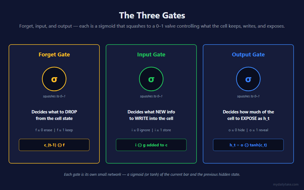
- Forget gate — for each cell neuron, a value near 1 keeps that memory, near 0 erases it. This is what lets the LSTM hold a value steady for many bars: keep the forget gate open and the cell state barely changes.
- Input gate — decides how much of the freshly proposed candidate actually gets written into the cell. Near 0 ignores the current bar; near 1 stores it.
- Output gate — decides how much of the cell state is exposed as the hidden state on this bar. The cell can hold information that the output gate keeps hidden until it becomes relevant.
The gates are not hand-coded rules — they are small networks trained alongside everything else. The model learns when to keep, write, and expose.
➡️ The Forward Step
StepCell advances both states by one bar — computing the four gates, updating the cell state, then the hidden state. OutputSigmoid reads the hidden state and produces P(up). The previous hidden state is snapshotted first so every neuron reads a consistent copy of it:
// One forward step. StepCell advances the hidden state h AND the cell state c
// by one bar:
//   f = sigmoid(Wxf.x + Whf.h_prev + bf)     forget gate
//   i = sigmoid(Wxi.x + Whi.h_prev + bi)     input gate
//   g = tanh   (Wxg.x + Whg.h_prev + bg)     candidate cell
//   o = sigmoid(Wxo.x + Who.h_prev + bo)     output gate
//   c <- f * c_prev + i * g                  new cell state
//   h <- o * tanh(c)                         new hidden state
// h_prev is snapshotted first so every neuron reads a consistent copy of it.

private void StepCell(double[] h, double[] c, double[] x)
{
    for (int j = 0; j < HiddenSize; j++) hPrevScratch[j] = h[j];

    for (int hh = 0; hh < HiddenSize; hh++)
    {
        double zf = bf[hh], zi = bi[hh], zg = bg[hh], zo = bo[hh];
        for (int k = 0; k < NumFeatures; k++)
        {
            double xk = x[k];
            zf += Wxf[hh][k] * xk;
            zi += Wxi[hh][k] * xk;
            zg += Wxg[hh][k] * xk;
            zo += Wxo[hh][k] * xk;
        }
        for (int j = 0; j < HiddenSize; j++)
        {
            double hj = hPrevScratch[j];
            zf += Whf[hh][j] * hj;
            zi += Whi[hh][j] * hj;
            zg += Whg[hh][j] * hj;
            zo += Who[hh][j] * hj;
        }
        double f  = Sigmoid(zf);
        double ig = Sigmoid(zi);
        double gg = Math.Tanh(zg);
        double og = Sigmoid(zo);
        double cv = f * c[hh] + ig * gg;
        c[hh] = cv;
        h[hh] = og * Math.Tanh(cv);
    }
}

// The output head reads the hidden state and produces P(up) via the sigmoid.

private double OutputSigmoid(double[] h)
{
    double z = by;
    for (int hh = 0; hh < HiddenSize; hh++) z += Wy[hh] * h[hh];
    return Sigmoid(z);
}
The live prediction calls StepCell once per bar on a persistent hidden and cell state that walk forward indefinitely. Training rebuilds a separate short walk from scratch — which is where backpropagation comes in.
🔁 Backpropagation Through the Gates
Training uses the same truncated Backpropagation Through Time as the RNN post: every training-eligible bar, the network is unrolled BpttWindow steps back, the forward pass through that sequence is recomputed, and the gradient is propagated backward through every step. The LSTM just has more to differentiate — four gates and two states per step instead of one:
// TRUNCATED BPTT — recompute the forward pass over the BpttWindow bars ending
// at trainBar, then backprop the gradient through every gate at every step.
// The anchor hidden + cell state at the start of the window is reset to zero
// each call — a standard simplification for online truncated BPTT.

private void TruncatedBptt(double y)
{
    // Forward pass over the window. hSeq[0]/cSeq[0] = zero anchor;
    // index t+1 = state after processing bar t. All gate activations are cached.
    for (int j = 0; j < HiddenSize; j++)
    {
        hSeq[0][j] = 0.0;
        cSeq[0][j] = 0.0;
    }
    for (int t = 0; t < BpttWindow; t++)
    {
        int ringIdx = LabelHorizon + BpttWindow - 1 - t;   // oldest first
        double[] xt = featureRing[ringIdx], hPrev = hSeq[t], cPrev = cSeq[t];
        double[] hCur = hSeq[t+1], cCur = cSeq[t+1];
        double[] fCur = fSeq[t+1], iCur = iSeq[t+1], gCur = gSeq[t+1], oCur = oSeq[t+1];
        for (int hh = 0; hh < HiddenSize; hh++)
        {
            double zf = bf[hh], zi = bi[hh], zg = bg[hh], zo = bo[hh];
            for (int k = 0; k < NumFeatures; k++)
            {
                double xk = xt[k];
                zf += Wxf[hh][k]*xk; zi += Wxi[hh][k]*xk;
                zg += Wxg[hh][k]*xk; zo += Wxo[hh][k]*xk;
            }
            for (int j = 0; j < HiddenSize; j++)
            {
                double hj = hPrev[j];
                zf += Whf[hh][j]*hj; zi += Whi[hh][j]*hj;
                zg += Whg[hh][j]*hj; zo += Who[hh][j]*hj;
            }
            double f = Sigmoid(zf), ig = Sigmoid(zi), gg = Math.Tanh(zg), og = Sigmoid(zo);
            double cv = f * cPrev[hh] + ig * gg;
            fCur[hh] = f; iCur[hh] = ig; gCur[hh] = gg; oCur[hh] = og;
            cCur[hh] = cv;
            hCur[hh] = og * Math.Tanh(cv);
        }
    }

    // Output, error, and seed gradients into the final hidden state.
    double error = OutputSigmoid(hSeq[BpttWindow]) - y;   // cross-entropy + sigmoid
    for (int hh = 0; hh < HiddenSize; hh++)
    {
        for (int k = 0; k < NumFeatures; k++)
        { gWxf[hh][k]=0; gWxi[hh][k]=0; gWxg[hh][k]=0; gWxo[hh][k]=0; }
        for (int j = 0; j < HiddenSize; j++)
        { gWhf[hh][j]=0; gWhi[hh][j]=0; gWhg[hh][j]=0; gWho[hh][j]=0; }
        gbf[hh]=0; gbi[hh]=0; gbg[hh]=0; gbo[hh]=0;
        gWy[hh]    = error * hSeq[BpttWindow][hh] + RegularizationLambda * Wy[hh];
        dhNext[hh] = error * Wy[hh];
        dcNext[hh] = 0.0;                         // no cell gradient from the future
    }
    double gby = error;

    // Walk backward through the unrolled time steps.
    //   doG = dh * tanh(c) ;  dc = dh * o * (1 - tanh(c)^2) + dcNext
    //   df = dc * c_{t-1} ;  di = dc * g ;  dg = dc * i ;  carry dc * f to t-1
    //   dz* = d* * (gate activation derivative)
    for (int t = BpttWindow; t >= 1; t--)
    {
        int ringIdx = LabelHorizon + BpttWindow - 1 - (t - 1);
        double[] xt = featureRing[ringIdx], hPrev = hSeq[t-1], cPrev = cSeq[t-1];
        double[] fCur = fSeq[t], iCur = iSeq[t], gCur = gSeq[t], oCur = oSeq[t], cCur = cSeq[t];

        for (int hh = 0; hh < HiddenSize; hh++)
        {
            double tanhC = Math.Tanh(cCur[hh]);
            double dh  = dhNext[hh];
            double doG = dh * tanhC;
            double dc  = dh * oCur[hh] * (1.0 - tanhC*tanhC) + dcNext[hh];
            double fv = fCur[hh], iv = iCur[hh], gv = gCur[hh], ov = oCur[hh];
            dcPrevScratch[hh] = dc * fv;          // cell gradient carried to t-1
            dzf[hh] = (dc * cPrev[hh]) * fv * (1.0 - fv);
            dzi[hh] = (dc * gv)        * iv * (1.0 - iv);
            dzg[hh] = (dc * iv)        * (1.0 - gv*gv);
            dzo[hh] = doG              * ov * (1.0 - ov);
        }

        for (int hh = 0; hh < HiddenSize; hh++)
        {
            double dzfh = dzf[hh], dzih = dzi[hh], dzgh = dzg[hh], dzoh = dzo[hh];
            for (int k = 0; k < NumFeatures; k++)
            {
                double xk = xt[k];
                gWxf[hh][k] += dzfh*xk; gWxi[hh][k] += dzih*xk;
                gWxg[hh][k] += dzgh*xk; gWxo[hh][k] += dzoh*xk;
            }
            for (int j = 0; j < HiddenSize; j++)
            {
                double hj = hPrev[j];
                gWhf[hh][j] += dzfh*hj; gWhi[hh][j] += dzih*hj;
                gWhg[hh][j] += dzgh*hj; gWho[hh][j] += dzoh*hj;
            }
            gbf[hh] += dzfh; gbi[hh] += dzih; gbg[hh] += dzgh; gbo[hh] += dzoh;
        }

        // Propagate dh/dc to the previous step (uses OLD recurrent weights).
        // Skipped at t == 1: hSeq[0]/cSeq[0] are the fixed zero anchor.
        if (t > 1)
        {
            for (int j = 0; j < HiddenSize; j++)
            {
                double s = 0.0;
                for (int hh = 0; hh < HiddenSize; hh++)
                    s += Whf[hh][j]*dzf[hh] + Whi[hh][j]*dzi[hh]
                       + Whg[hh][j]*dzg[hh] + Who[hh][j]*dzo[hh];
                dhPrevScratch[j] = s;
            }
            for (int j = 0; j < HiddenSize; j++)
            { dhNext[j] = dhPrevScratch[j]; dcNext[j] = dcPrevScratch[j]; }
        }
    }

    // Apply weight updates — plain SGD, L2 on the weight matrices only.
    for (int hh = 0; hh < HiddenSize; hh++)
    {
        for (int k = 0; k < NumFeatures; k++)
        {
            Wxf[hh][k] -= LearningRate * (gWxf[hh][k] + RegularizationLambda * Wxf[hh][k]);
            Wxi[hh][k] -= LearningRate * (gWxi[hh][k] + RegularizationLambda * Wxi[hh][k]);
            Wxg[hh][k] -= LearningRate * (gWxg[hh][k] + RegularizationLambda * Wxg[hh][k]);
            Wxo[hh][k] -= LearningRate * (gWxo[hh][k] + RegularizationLambda * Wxo[hh][k]);
        }
        for (int j = 0; j < HiddenSize; j++)
        {
            Whf[hh][j] -= LearningRate * (gWhf[hh][j] + RegularizationLambda * Whf[hh][j]);
            Whi[hh][j] -= LearningRate * (gWhi[hh][j] + RegularizationLambda * Whi[hh][j]);
            Whg[hh][j] -= LearningRate * (gWhg[hh][j] + RegularizationLambda * Whg[hh][j]);
            Who[hh][j] -= LearningRate * (gWho[hh][j] + RegularizationLambda * Who[hh][j]);
        }
        bf[hh] -= LearningRate * gbf[hh];
        bi[hh] -= LearningRate * gbi[hh];
        bg[hh] -= LearningRate * gbg[hh];
        bo[hh] -= LearningRate * gbo[hh];
        Wy[hh] -= LearningRate * gWy[hh];
    }
    by -= LearningRate * gby;
}
The backward pass carries two gradients between steps: one for the hidden state and one for the cell state. At each step the cell gradient picks up a contribution from the hidden path (through the output gate and the tanh) and a contribution carried straight back from the next step’s forget gate — and that second path is the important one, as the next section shows.
Two honest notes, the same as the RNN post. First, at the start of each training window the anchor hidden state and cell state are both reset to zero, rather than carried from the live model’s actual state at that bar — a standard simplification for online truncated BPTT that keeps every training step self-contained. Second, the weight update here is plain stochastic gradient descent — one update per training-eligible bar. The Adam optimizer from Post 5 could be layered on unchanged; it is left out so the gradient flow through the gates stays the focus.
🛣️ The Gradient Highway
Here is the payoff — why all the gate machinery is worth it. Recall the vanilla RNN’s problem: every backward step multiplied the gradient by a tanh derivative, a number around 0.5, and ten of those in a row left almost nothing. Now look at the LSTM’s cell-state path.
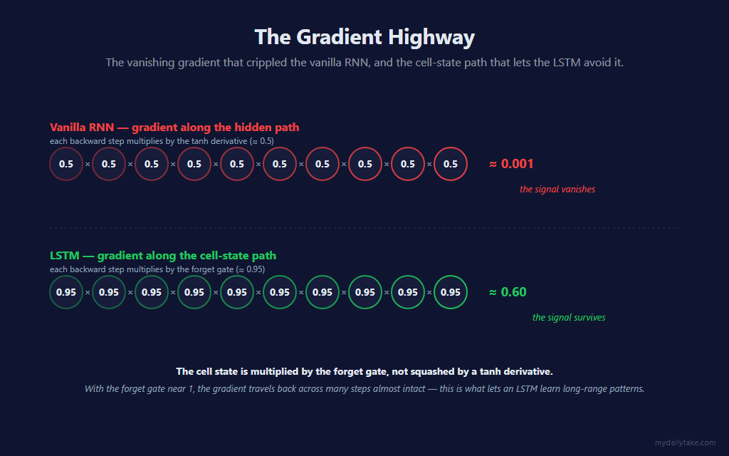
The cell update is c_t = f ⊙ c_{t-1} + i ⊙ g. Differentiate it with respect to the previous cell state and the answer is just f — the forget gate. So on the backward pass, the gradient travelling along the cell state is multiplied by the forget gate at each step, not by a tanh derivative. The forget gate is learned, and it commonly sits close to 1 (the indicator even initializes its bias positive so it starts that way). A chain of numbers near 1 barely decays — ten steps of ×0.95 still leaves ~60% of the signal, against the RNN’s ~0.1%.
That uninterrupted path is sometimes called the constant error carousel. It is the core reason the LSTM can learn long-range dependencies: the gradient actually reaches the early bars of the window with enough strength to update the weights there.
🎚️ Why a Wider BpttWindow Pays Off
In the RNN post, widening BpttWindow from 3 to 25 barely changed anything — the gradient had vanished long before it reached those extra bars, so they contributed almost nothing. The LSTM changes that calculus:
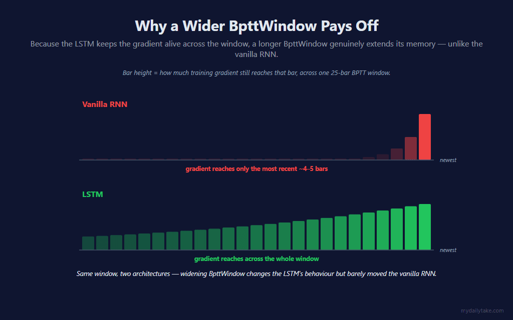
Because the cell-state path keeps the gradient alive, every bar inside the window receives a training signal worth something — so a longer BpttWindow genuinely extends the model’s memory rather than just costing compute. The trade-off is real but different from the RNN’s: a wider window here means more useful learning and proportionally more work per training step. The default of 10 is a reasonable balance; raising it is a defensible choice with this architecture in a way it never was with the vanilla RNN.
🔧 The Training Loop
Each bar runs four steps in order: advance the live hidden and cell state for the prediction, push the new feature vector into a rolling ring buffer, run one truncated-BPTT step if a label is now observable, and publish the outputs. The ring buffer is sized exactly BpttWindow + LabelHorizon — enough history to rebuild the window and reach the bar whose outcome is now known:
// Inside OnBarUpdate, after the feature vector for the current bar is built.
// Four steps run in order on every bar:

// 1) Live forward step — advance the persistent hidden + cell state, read P(up).
NormalizeInto(scratchNorm, scratchRaw, 0);
StepCell(hLive, cLive, scratchNorm);     // h and c advance one LSTM step
double pUp = OutputSigmoid(hLive);

// 2) Push the new normalized feature into the ring buffer (index 0 = newest).
//    The ring is sized BpttWindow + LabelHorizon — exactly enough history.
PushFeatureRing(scratchNorm);

// 3) Training step — once the buffer holds a full BPTT window AND the bar
//    from LabelHorizon ago has an observable forward outcome.
int needForTraining = BpttWindow + LabelHorizon;
if (ringFilled >= needForTraining && CurrentBar >= predictionWarmup + LabelHorizon)
{
    int    trainBar     = LabelHorizon;
    bool   trainThisBar = false;
    double y            = 0.0;

    if (LabelMode == MlNeuralNetLstm_LabelMode.CloseToClose)
    {
        y = Close[0] > Close[trainBar] ? 1.0 : 0.0;
        trainThisBar = true;
    }
    // (FavorableExcursion branch omitted here — see the Label Mode setting.)

    if (trainThisBar)
        TruncatedBptt(y);                // one truncated-BPTT update through the gates
}

// 4) Publish the public-Series outputs for downstream strategies.
sProbabilityUp[0] = pUp;
sConfidence[0]    = Math.Abs(pUp - 0.5) * 2.0;
The look-ahead safety is unchanged from the rest of the series: the model trains on the bar from LabelHorizon ago — whose realized direction is now genuinely observable — and predicts on the current bar. Nothing in the training path reads a price the live model would not have had.
📊 What This Looks Like on a Chart
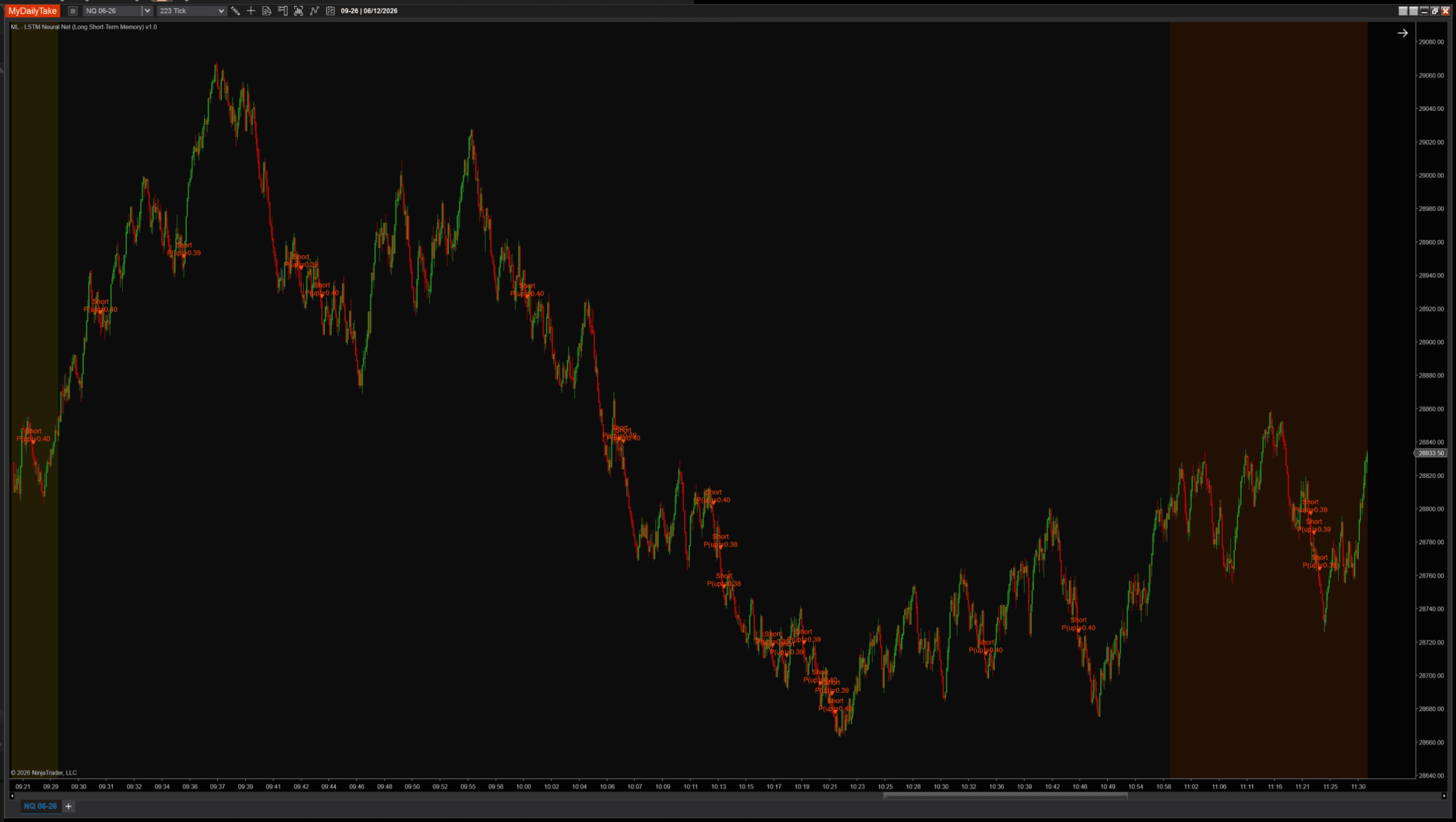
Same indicator, same NQ session, same features and labels. Only BpttWindow changes. Start with the default:
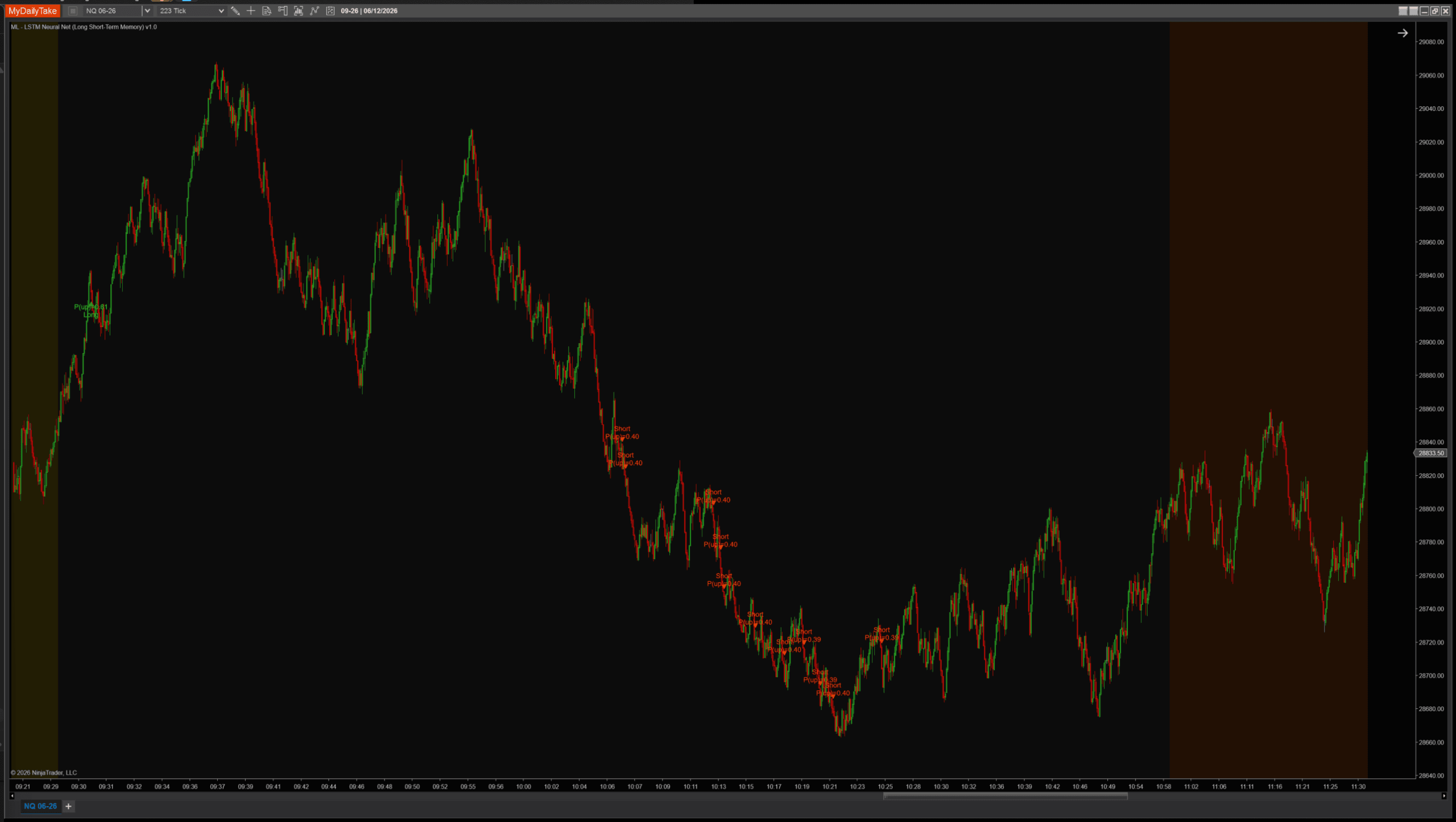
Default settings (BpttWindow = 10). A moderate, clustered set of signals.
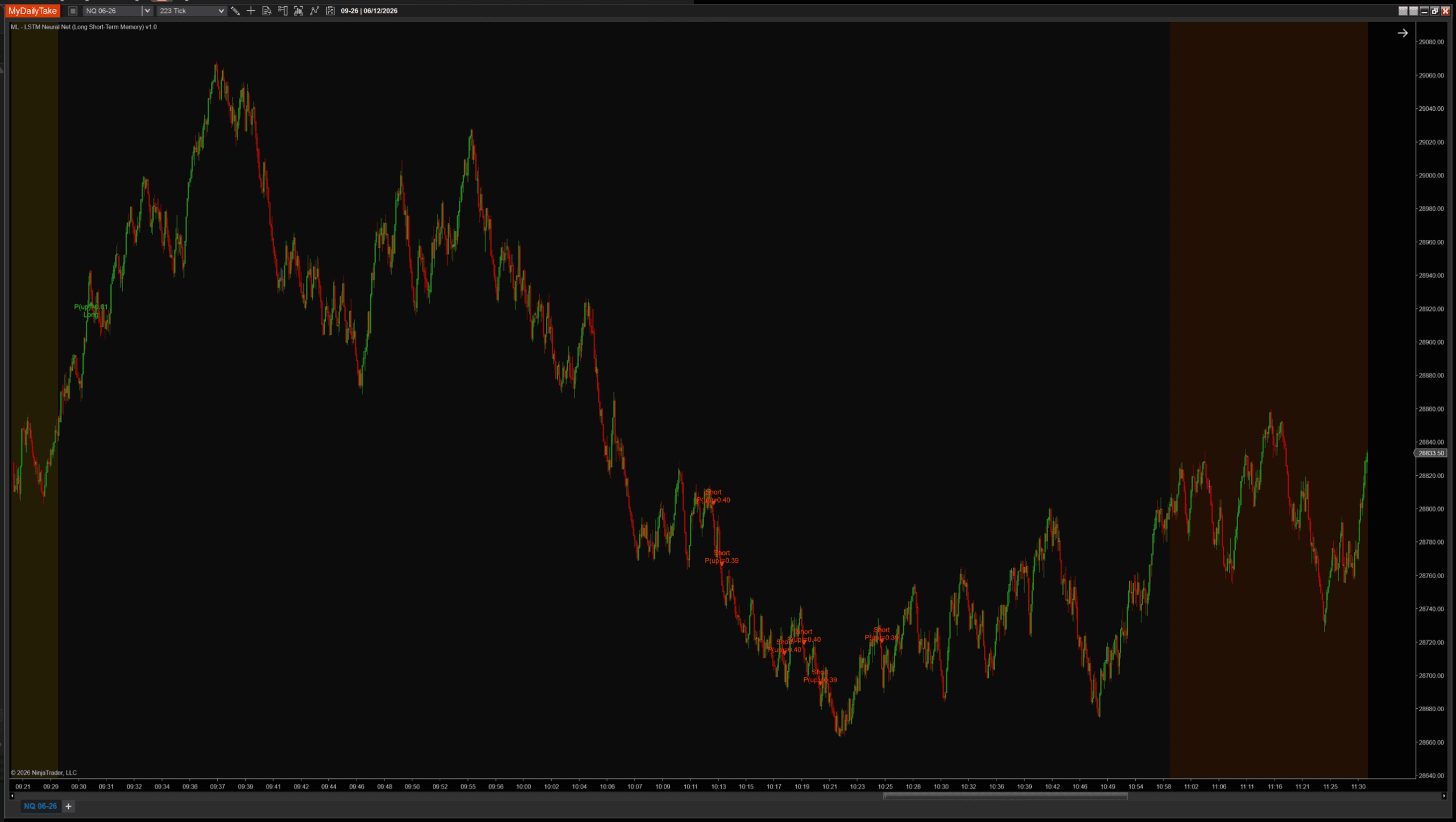
BpttWindow = 3 (short memory). The most signals of the three.
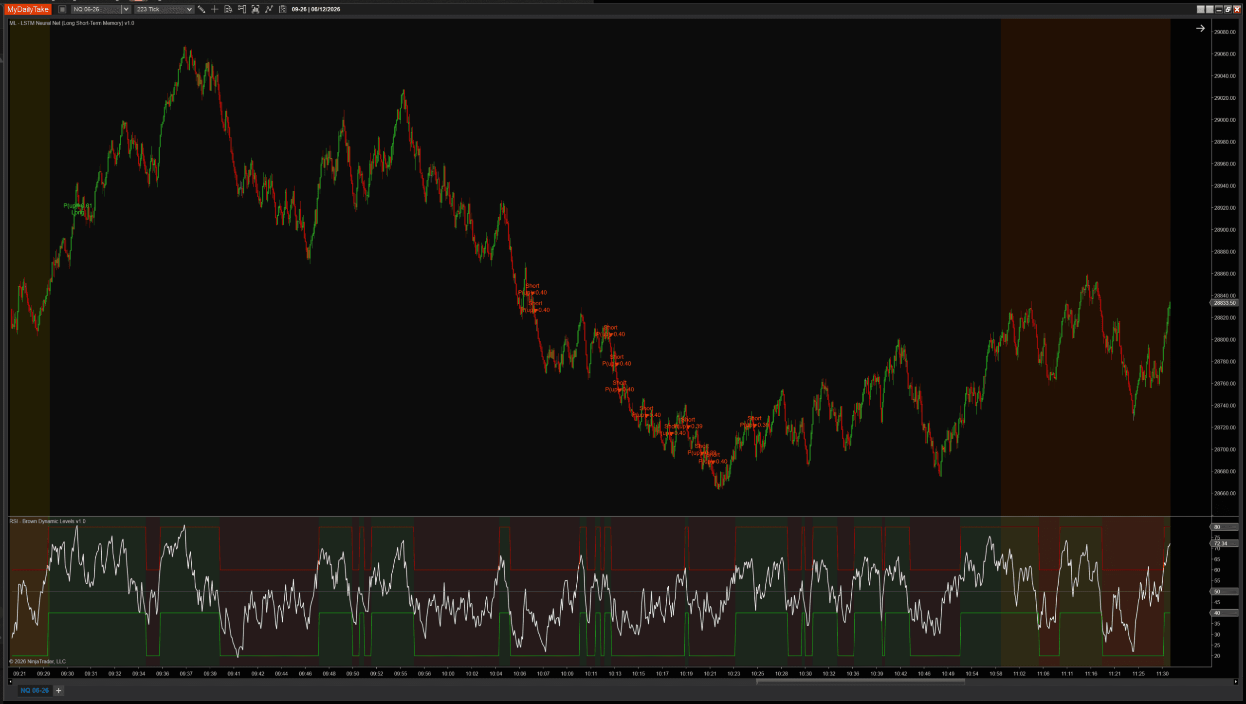
BpttWindow = 25 (long memory). Markedly more selective — far fewer signals.
This is the contrast the RNN post could not show. There, three windows spanning 3 to 25 bars produced near-identical charts. Here the signal set visibly changes — and in a consistent direction: the wider the window, the fewer and more selective the signals.
That direction is worth understanding, because it is the same effect you will see if you simply load more history. A wider BpttWindow feeds more context into every training step; more effective training on a genuinely hard, noisy target — directional prediction from three features — produces a better-calibrated model. Cross-entropy training is a proper scoring rule: it pushes the model toward honest probabilities, and an honest model on a low-signal problem outputs values close to 0.5. Fewer of those clear the Min Probability Edge gate, so fewer signals fire. The short-window model is noisier and more reactive — more signals, but from a model that has trained on less context per step. If you want a steady signal count regardless of window or history length, the lever is Min Probability Edge, not the window.
⚙️ Settings
The indicator’s settings are grouped into five categories. Architecture sets the network shape and the BPTT window. Learning controls the labeling and the L2 penalty. Features controls what the model sees. Signal controls when triangles fire. Display is cosmetic-only.
Architecture
| Parameter | Description |
|---|---|
| Hidden Size | Number of neurons in the LSTM hidden layer. Each bar updates an H-dimensional hidden-state vector AND an H-dimensional cell-state vector — together they are the network's memory. Larger H = more capacity but more parameters; the LSTM has four gates, so roughly 4x the weights of a vanilla RNN of the same size. Default 8. |
| BPTT Window (bars) | Number of past bars the network is unrolled through when computing gradients (truncated Backpropagation Through Time). Bigger window = the model can learn longer-range dependencies. Unlike the vanilla RNN, the LSTM's cell-state path keeps gradients alive across longer windows, so a larger BpttWindow is genuinely more worthwhile here — at a proportional compute cost per training step. Default 10. |
| Random Seed | Seed for the random weight initialization (when Weight Init = Random). The same seed produces the same starting weights — useful for reproducible testing or comparing settings fairly. |
Learning
| Parameter | Description |
|---|---|
| Learning Rate | Step size for each weight update. LSTM training is sensitive to learning rate because gradients compound across the BPTT window and four gates. Start at 0.005 and lower it first if training looks unstable. |
| Regularization Lambda (L2) | L2 penalty on weight magnitude. Pulls weights gently toward zero each update so they don't drift to extreme values. Applied to the gate weight matrices only, not the biases. Recommended 0.0001 to 0.001; default 0.0005. |
| Label Horizon (bars) | How many bars ahead the realized direction is observed. The model updates each bar using the prediction from N bars ago, whose forward outcome is now known — this keeps training look-ahead-safe. |
| Weight Init | Zero starts every weight at 0 — but then all four gates would be identical and nothing could propagate (the symmetry problem). Random is strongly recommended; it uses Xavier/Glorot scaling for the gate weights and starts the forget-gate bias positive (1.0) so the cell remembers by default early in training. |
| Label Mode | How the training label is defined. CloseToClose: y = 1 if Close at the end of the Label Horizon window is above Close at the training bar. FavorableExcursion: y = 1 if the long-side favorable move beat the short-side move during the window (uses bar highs/lows); bars below Min Favorable Move are skipped as chop. |
| Min Favorable Move (ATRs) | ONLY USED WHEN Label Mode = FavorableExcursion. Minimum favorable excursion (in ATRs at entry) required during the post-bar window for the model to update on that bar. |
Features
| Parameter | Description |
|---|---|
| MA Period | Period of the moving average used in the distance-from-MA feature, and the smoothing window for the ATR regime-ratio feature. |
| ATR Period | Period of the ATR used to scale every feature into volatility units, so distance comparisons stay consistent across regimes. |
| Slope Lookback (bars) | Number of bars over which the slope feature is measured: (Close[0] − Close[N]) / ATR. |
| Normalize Features (Z-Score) | Master toggle for z-score normalization. When ON, each feature is rescaled against its own historical rolling stats. Recommended ON. |
| Normalization Lookback (bars) | Window used to compute the rolling mean and standard deviation that z-score the features. Each bar uses its own local-time stats. |
Signal
| Parameter | Description |
|---|---|
| Min Probability Edge | How far the predicted probability of an up move must be from 0.5 before a signal fires. 0.10 means a long fires when P(up) > 0.60 and a short fires when P(up) < 0.40. |
| Signal Cooldown (bars) | Minimum number of bars between consecutive signals. Higher values space signals out so the chart stays readable. |
Display
| Parameter | Description |
|---|---|
| Marker Offset (ticks) | Vertical offset of the signal triangle from the bar's high (shorts) or low (longs), in ticks. |
| Label Offset (ticks) | Distance from the bar to the text label, in ticks. Should be larger than Marker Offset so the label sits beyond the triangle. |
| Show Labels | Render the predicted-probability label beside each signal triangle. |
| Label Font Size | Font size for the signal labels. |
As in the RNN post, Learning Rate deserves care: gradients compound across the BPTT window and four gates, so the default of 0.005 is deliberately conservative. If signals flicker wildly bar to bar, lower it before changing anything else.
🎚️ Pairing With a Regime Filter
Same defensive pattern as the prior posts. An RSI(14) above or below 50 vetoes counter-trend signals, so the model is only allowed to fire in the direction of the broader trend:
The LSTM’s raw signal is a probability; the regime filter is a separate, far simpler model. Combining a learned signal with a transparent rule-based veto is a dependable way to keep an online learner from fighting the obvious trend.
🛠️ Using It in a Strategy
The indicator exposes its outputs as public Series so a strategy can consume the model directly:
Public Outputs
| Output | Type | Purpose |
|---|---|---|
| ProbabilityUpSeries |
Series | The model's predicted probability of an up move — the post-sigmoid output. Range [0, 1]. |
| ConfidenceSeries |
Series | |P(up) − 0.5| × 2 — distance from a coin-flip, scaled to [0, 1]. 0 = uncertain, 1 = maximum conviction. |
| IsLongSignalSeries |
Series | True on bars where the prediction passes the probability gate AND the cooldown — a long signal fires. |
| IsShortSignalSeries |
Series | True on bars where the prediction passes the probability gate AND the cooldown — a short signal fires. |
Below is a working strategy that combines the model’s signal with the RSI regime filter from the previous section — a long is allowed only when the model predicts up and RSI is above 50, and the mirror for shorts:
private MlNeuralNetLstm     nn;
private RSI                 rsi;

protected override void OnStateChange()
{
    if (State == State.SetDefaults)
    {
        Name        = "LstmRsiTrendFollower";
        Calculate   = Calculate.OnBarClose;
    }
    else if (State == State.DataLoaded)
    {
        nn = MlNeuralNetLstm(
            hiddenSize:             8,
            bpttWindow:             10,
            randomSeed:             42,
            learningRate:           0.005,
            regularizationLambda:   0.0005,
            labelHorizon:           2,
            weightInit:             MlNeuralNetLstm_WeightInitMode.Random,
            labelMode:              MlNeuralNetLstm_LabelMode.CloseToClose,
            minFavorableMoveAtrs:   1.0,
            maPeriod:               8,
            atrPeriod:              50,
            slopeLookback:          2,
            normalizeFeatures:      true,
            normalizationLookback:  200,
            minProbabilityEdge:     0.10,
            signalCooldownBars:     3);

        rsi = RSI(14, 3);
    }
}

protected override void OnBarUpdate()
{
    // The indicator gates its own signals through warmup; this is a safety margin.
    if (CurrentBar < 350) return;

    // Long: model predicts up AND RSI confirms the uptrend regime.
    if (nn.IsLongSignalSeries[0] && rsi[0] > 50)
        EnterLong("NN Long");

    // Short: model predicts down AND RSI confirms the downtrend regime.
    if (nn.IsShortSignalSeries[0] && rsi[0] < 50)
        EnterShort("NN Short");
}
📝 The Honest Validation Talk (Still)
The LSTM is the most expressive model in this series so far — two states, four gates, and a memory that can reach back many bars. More expressiveness means more capacity to fit noise, not just signal. And the chart section above is a live demonstration of why evaluation is hard: the same model, on the same data, produces a different signal set depending on a single training hyperparameter — because an online learner is a moving target whose behavior depends on how, and how much, it has been trained. “Accuracy over the last N bars” averages over many effective models. None of that is a reason to avoid the LSTM; it is a reason to evaluate it honestly. Walk-forward across multiple regimes is still the only honest evaluation, and the work scales with how seriously you intend to trust the result.
📦 Download
Install:
- Download the .zip file above.
- In NinjaTrader 8, go to Tools → Import → NinjaScript Add-On.
- Select the downloaded .zip file.
- The indicator will appear under Indicators → indMyDailyTake → ML – LSTM Neural Net (Long Short-Term Memory) v1.0 on your chart.


This is the seventh installment of the Learn NinjaScript ML series. Post 1 covered k-Nearest Neighbors, Post 2 online logistic regression, Post 3 added a single hidden layer, Post 4 extended to configurable depth, Post 5 added the Adam optimizer, and Post 6 built a vanilla recurrent network — and ran into the vanishing gradient. Post 7 (this one) fixed it with the LSTM’s gated cell state.