ML — Multi-Hidden-Layer Neural Network: Configurable Depth in NinjaTrader 8
The prior post built a single-hidden-layer neural network — three inputs, six tanh neurons in one hidden layer, one sigmoid output, 31 parameters. It worked because the hidden layer can compose the raw features into non-linear combinations that a single neuron cannot represent. The post closed with a hint: “add a hidden layer + backprop and unlock non-linear feature interactions a single neuron cannot represent.” This post takes the next step — what happens when you add more hidden layers?
The same indicator is now configurable to any depth. Set HiddenLayerSizes to 6 for one hidden layer (matches the prior post), 8, 6 for two layers, 10, 6, 4 for three. The parser accepts any common separator — comma, space, hyphen, semicolon, x. Each new layer composes the previous one’s outputs into higher-order patterns. But more layers also bring new costs: vanishing gradients, more parameters than your data can train, and diminishing returns. This post unpacks all three.
📐 The Depth Spectrum
One hidden layer, two, or three — all using the same three trend-following features as the prior posts (distFromMa, slope, atrRegime) and the same online-learning loop. The only thing that changes is the architecture string:
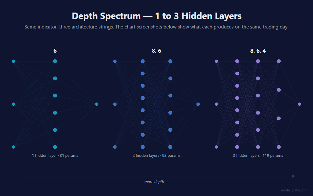
Each additional layer is a new matrix of weights that gets composed on top of the layer before it. Layer 1 detects combinations of raw features. Layer 2 composes layer-1 features into higher-order patterns. Layer 3, if you have one, composes those further. That’s the architectural promise of depth — compositional capacity.
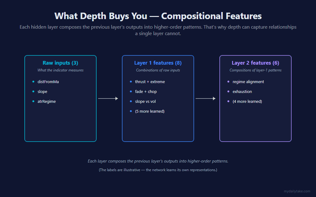
The labels in the diagram above are illustrative — the network isn’t told to learn “thrust + extreme.” It just learns whatever combinations minimize the prediction error. But the structure is real: each hidden layer’s neurons see the previous layer’s outputs and combine them, the way the first hidden layer combined the raw inputs.
⚖️ The Catch: Vanishing Gradients
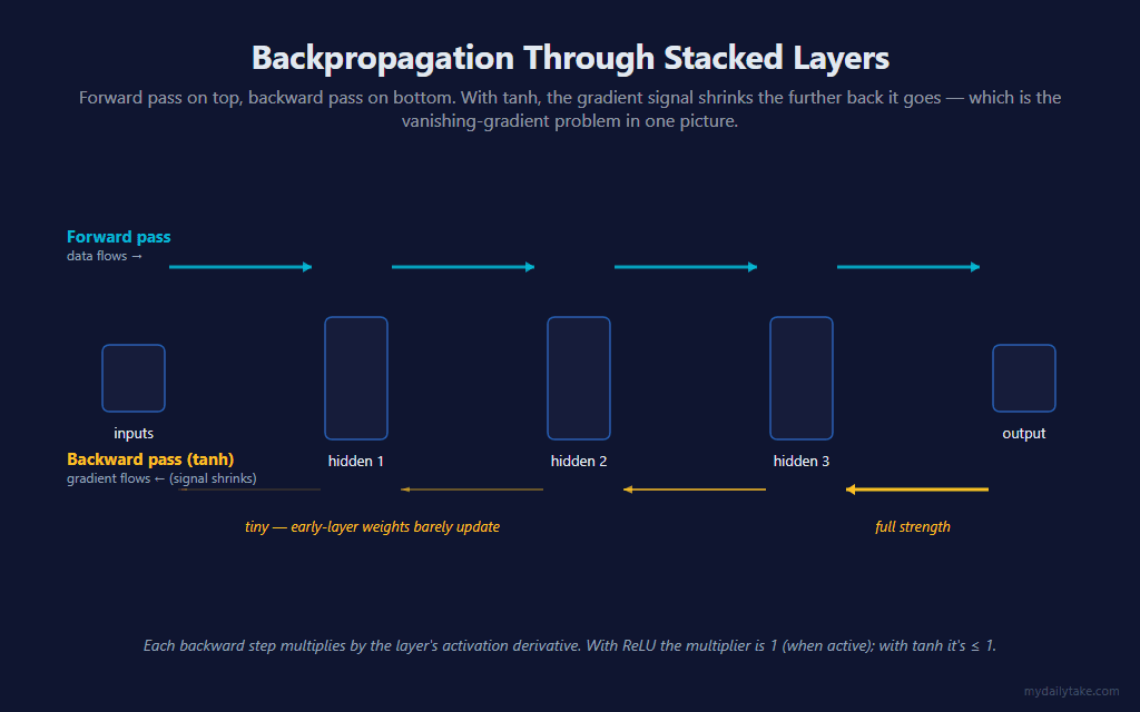
Backprop propagates the prediction error backward through the network by multiplying it through each layer’s activation derivative. The derivative is at most 1. With tanh, it’s usually closer to 0.5 in the responsive region; sigmoid caps at 0.25. So with three tanh layers, the gradient signal reaching the earliest layer’s weights is roughly 0.5 × 0.5 × 0.5 = 0.125 — eight times smaller than the gradient at the output side. The earliest layer barely updates.
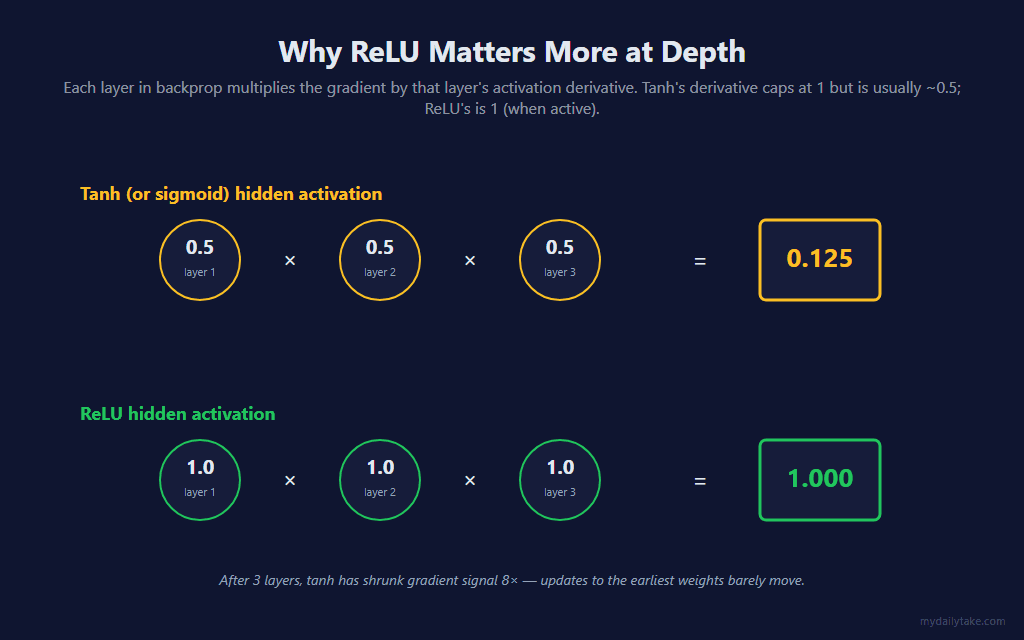
ReLU avoids this. Its derivative is 1 when the neuron is active (pre-activation > 0) and 0 when it isn’t. The chain-rule product through ReLU layers is 1 × 1 × 1 = 1 — full strength preserved through depth. This is why ReLU became the default for deep networks and why we set ReLU as the default activation in this indicator (the prior post defaulted to tanh because at a single hidden layer the difference doesn’t matter much).
➡️ The Forward Pass, Generalized
The forward pass is the same idea as the single-hidden-layer version, just looped over an arbitrary number of layers. For each layer, dot-product the inputs (or the previous layer’s activations) with the layer’s weights, add the biases, run through the activation. Cache the intermediates so the backward pass can reuse them.
// Forward pass — runs every bar to compute P(up).
// inputs (NumFeatures) -> layer 0 -> layer 1 -> ... -> output sigmoid.
// Caches every layer's pre- and post-activation values so the backward pass
// can compute gradients without re-running the forward pass.

private double ForwardPass(double[] inputs)
{
    for (int l = 0; l < numHiddenLayers; l++)
    {
        double[] inputToLayer = (l == 0) ? inputs : hiddenAct[l - 1];
        int sizeIn  = inputToLayer.Length;
        int sizeOut = layerSizes[l];

        for (int h = 0; h < sizeOut; h++)
        {
            double z = bh[l][h];
            for (int k = 0; k < sizeIn; k++)
                z += Wh[l][h][k] * inputToLayer[k];
            hiddenPre[l][h] = z;
            hiddenAct[l][h] = Activate(z);
        }
    }

    // Output layer reads from the last hidden layer.
    int last = numHiddenLayers - 1;
    double zOut = bo;
    for (int h = 0; h < layerSizes[last]; h++)
        zOut += Wo[h] * hiddenAct[last][h];

    return Sigmoid(zOut);
}
The first iteration of the outer loop uses the raw normalized inputs. Every subsequent iteration uses the prior layer’s hiddenAct array as its input. The output layer is hardcoded to a single sigmoid neuron because we’re producing a probability — same as the prior posts.
⬅️ Backprop Through Stacked Layers
Backprop is also generalized — it walks backward from the last hidden layer to the first, computing each layer’s gradient using the gradient flowing in from the layer ahead of it (the chain rule, made literal).
The critical detail: when propagating the gradient from layer l to layer l-1, we must use the old values of Wh[l] — the weights as they were during the forward pass. If we updated Wh[l] first and then computed dHiddenAct[l-1] using the new weights, the chain rule would be subtly wrong (we’d be computing the gradient of a different network than the one whose error we’re trying to back-propagate). The loop body below preserves the correct order: compute backward signals first, then update.
// Backprop — chain-rule gradient descent through every hidden layer.
// Cross-entropy loss + sigmoid output simplifies dL/dzOut to (pTrain - y).
// Walking backward from the last hidden layer to the first:
//   1. Convert dHiddenAct[l] to dHiddenPre[l] via activation derivative.
//   2. If a layer below exists, propagate dHiddenAct[l-1] using the OLD Wh[l].
//   3. Update Wh[l] and bh[l].
// Output weights Wo and bo are updated last.

private void Backprop(double[] inputs, double pTrain, double y)
{
    double error = pTrain - y;   // dL/dzOut for cross-entropy + sigmoid

    int last = numHiddenLayers - 1;

    // Seed gradient at the last hidden layer's activations from the output side.
    for (int h = 0; h < layerSizes[last]; h++)
        dHiddenAct[last][h] = error * Wo[h];

    // Walk backward through the hidden layers.
    for (int l = last; l >= 0; l--)
    {
        int sizeOut = layerSizes[l];
        int sizeIn  = (l == 0) ? NumFeatures : layerSizes[l - 1];
        double[] inputToLayer = (l == 0) ? inputs : hiddenAct[l - 1];

        for (int h = 0; h < sizeOut; h++)
            dHiddenPre[l][h] = dHiddenAct[l][h] * ActivationDerivative(hiddenPre[l][h], hiddenAct[l][h]);

        // Propagate to dHiddenAct[l-1] using the OLD Wh[l] — must happen BEFORE updating.
        if (l > 0)
        {
            for (int k = 0; k < sizeIn; k++) dHiddenAct[l - 1][k] = 0;
            for (int h = 0; h < sizeOut; h++)
            {
                double dpre = dHiddenPre[l][h];
                for (int k = 0; k < sizeIn; k++)
                    dHiddenAct[l - 1][k] += dpre * Wh[l][h][k];
            }
        }

        // Now update Wh[l] and bh[l].
        for (int h = 0; h < sizeOut; h++)
        {
            double dpre = dHiddenPre[l][h];
            for (int k = 0; k < sizeIn; k++)
            {
                double grad = dpre * inputToLayer[k] + RegularizationLambda * Wh[l][h][k];
                Wh[l][h][k] -= LearningRate * grad;
            }
            bh[l][h] -= LearningRate * dpre;
        }
    }

    // Update output layer weights and bias.
    for (int h = 0; h < layerSizes[last]; h++)
    {
        double gradWo = error * hiddenAct[last][h] + RegularizationLambda * Wo[h];
        Wo[h] -= LearningRate * gradWo;
    }
    bo -= LearningRate * error;
}
That four-step inner loop — compute dHiddenPre, propagate to dHiddenAct[l-1] if a layer below exists, then update Wh[l] and bh[l] — is the structural heart of every neural-network library, just written without the abstraction. Whether the network has 1, 2, 3, or 30 hidden layers, this loop is what runs.
⚖️ Two Ways to Label a Bar (Same as Before)
The label rule is the same parameter as the prior posts — LabelMode — and the trade-off between the two modes hasn’t changed:
- CloseToClose:
y = 1ifClose[0] > Close[trainBar]. Tracks pure close-to-close direction. Trains on every observable bar. - FavorableExcursion:
y = 1if max favorable excursion in the LONG direction beat the SHORT direction during the window. Skips bars belowMinFavorableMoveAtrs— chop bars don’t train.
The choice of label still defines what the model is trying to predict, and that choice still matters more than the architecture. A 119-parameter three-layer network with a poorly-chosen label rule will lose to a 31-parameter single-layer network with a thoughtful one. Depth does not rescue you from labeling the wrong target.
🔁 The Update Step
The update logic is unchanged from the prior post — compute the label using the bar from LabelHorizon ago, do a forward pass at that bar, run one step of backprop. The only difference is that “one step of backprop” now propagates the error through all N hidden layers instead of just one.
// Update step — runs every bar (when training conditions are met).
// Uses the bar from LabelHorizon ago, whose forward outcome is now observable.
int trainBar = LabelHorizon;
bool   trainThisBar = false;
double y            = 0.0;

if (LabelMode == MlNeuralNetMultiLayer_LabelMode.CloseToClose)
{
    y = Close[0] > Close[trainBar] ? 1.0 : 0.0;
    trainThisBar = true;
}
else // FavorableExcursion: y = 1 if MFE_long > MFE_short during the window.
{
    double closeAtTrain = Close[trainBar];
    double safeAtrTrain = atr[trainBar] > 1e-9 ? atr[trainBar] : TickSize;

    double maxHigh = double.MinValue;
    double minLow  = double.MaxValue;
    for (int b = 0; b < LabelHorizon; b++)
    {
        if (High[b] > maxHigh) maxHigh = High[b];
        if (Low[b]  < minLow)  minLow  = Low[b];
    }

    double mfeLong  = (maxHigh    - closeAtTrain) / safeAtrTrain;
    double mfeShort = (closeAtTrain - minLow)     / safeAtrTrain;

    if (Math.Max(mfeLong, mfeShort) >= MinFavorableMoveAtrs)
    {
        y = mfeLong > mfeShort ? 1.0 : 0.0;
        trainThisBar = true;
    }
}

if (trainThisBar)
{
    GetFeaturesInto(scratchRaw, trainBar);
    NormalizeInto(scratchNorm, scratchRaw, trainBar);

    // Forward pass at trainBar with current weights, then one backprop step.
    double pTrain = ForwardPass(scratchNorm);
    Backprop(scratchNorm, pTrain, y);
}
Look-ahead safety is preserved by the same mechanism: predictions on the current bar use weights last updated from a bar LabelHorizon ago, so the model has never seen the future.
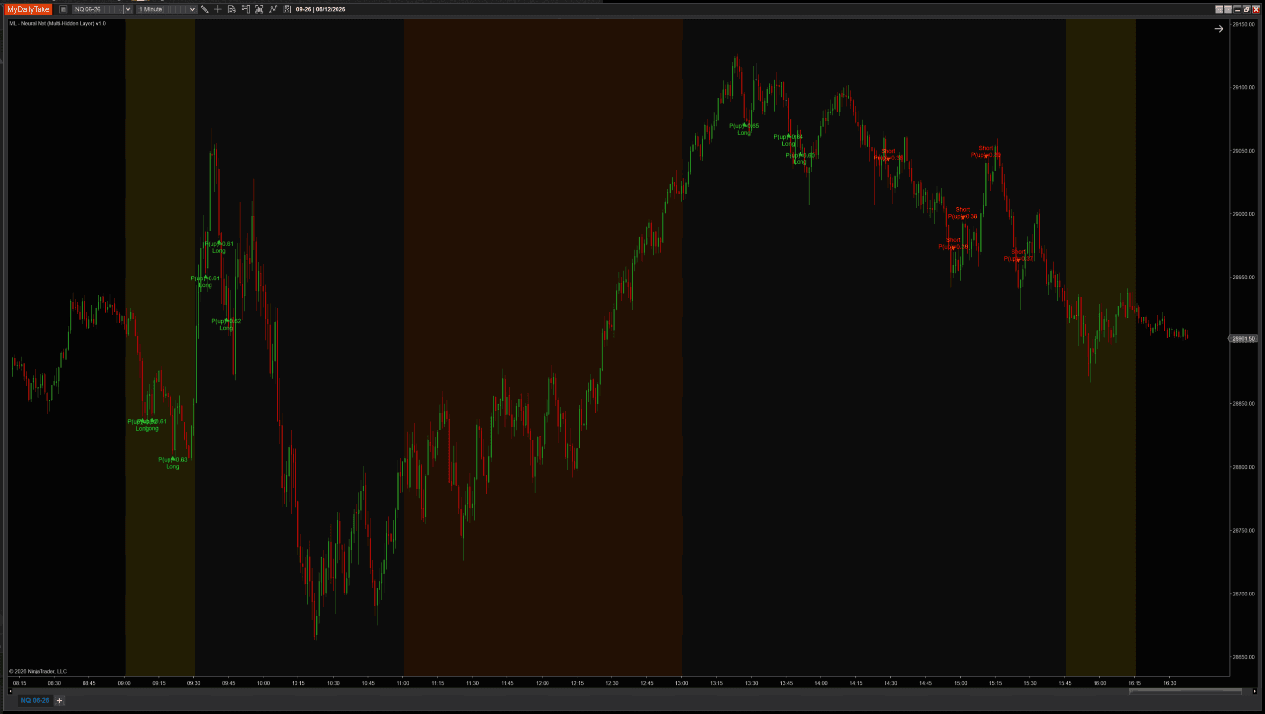
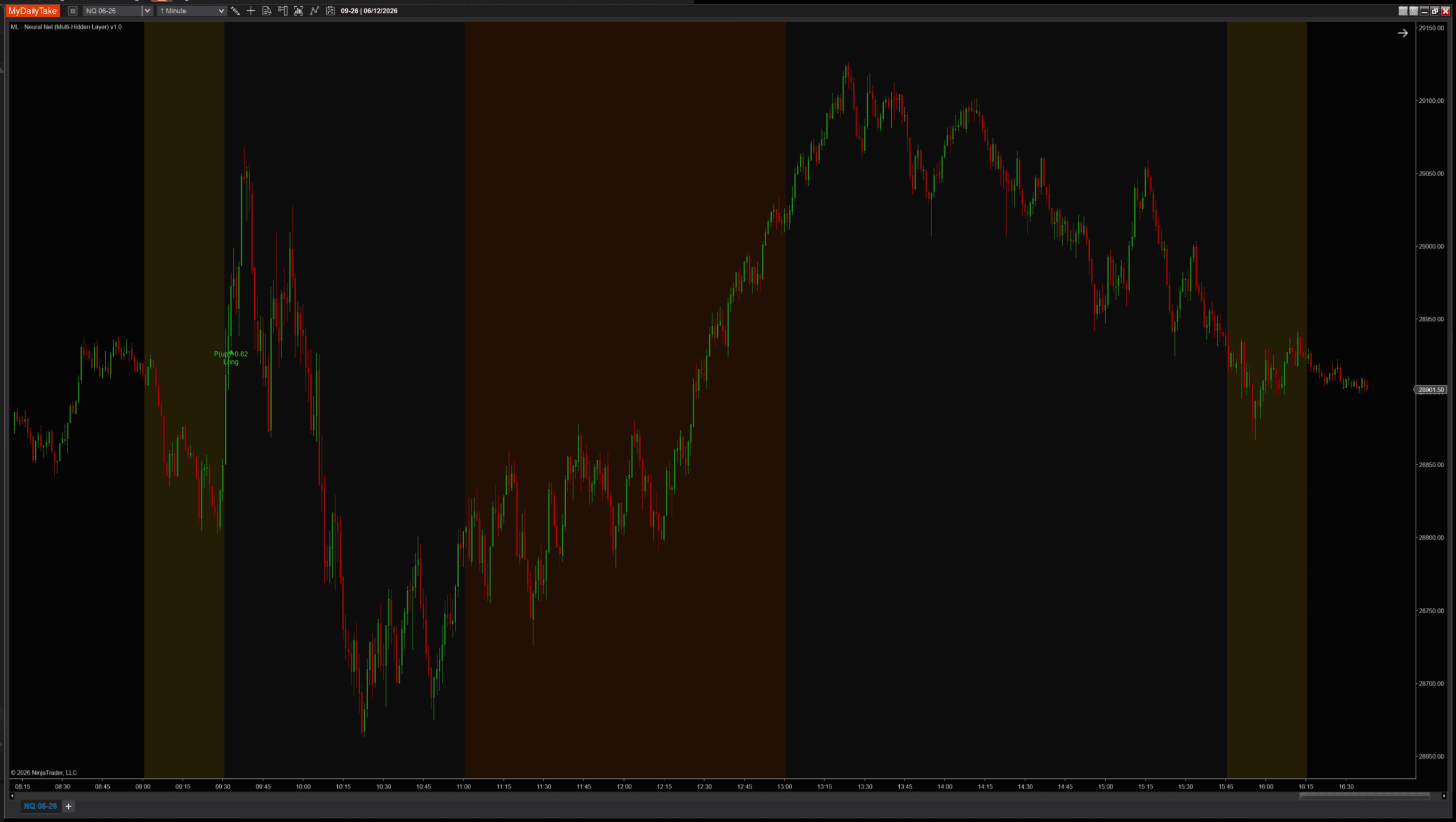
📊 What This Looks Like on a Chart
Below: the same trading session, same indicator, same all other settings — only HiddenLayerSizes changing. One layer of 6 neurons (matches the prior post), two layers (default for this post), three layers.
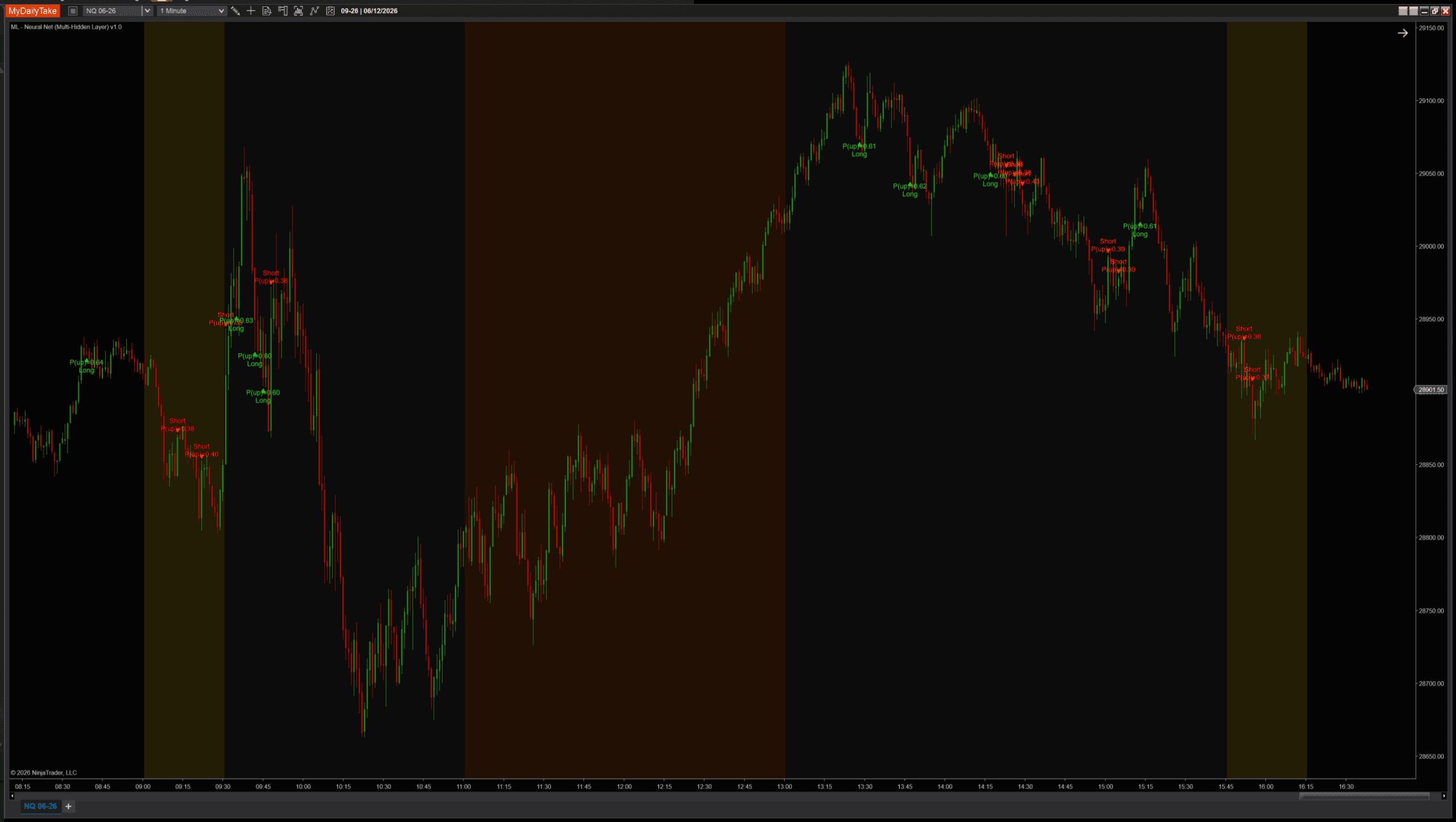
One hidden layer of 6 (matches the prior post). Many signals across the day.
Two hidden layers (8 then 6). Fewer, more selective signals.
Three hidden layers (8 then 6 then 4). Only one signal fires the entire session — the deeper network is under-trained at this depth on a single day’s bars.
That third chart is the practical lesson of this post: more depth is not always better. The three-layer network has 119 parameters; with the small amount of training data a single session provides, those parameters never get enough gradient signal to settle into a confident prediction. The model could probably learn richer patterns than the shallower architectures — but only if it had more data to learn from.
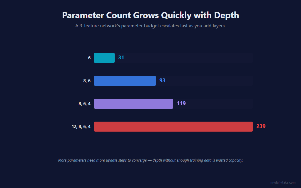
The parameter count escalates fast. With 3 input features, a two-layer (8, 6) network is already near the practical sweet spot — enough capacity to learn meaningful feature compositions, few enough parameters that the gradient signal stays strong and the model converges within a session’s worth of bars.
💪 Where Depth Helps, and Where It Doesn’t
Depth helps when the underlying relationships in the data are compositional — when there’s a “feature of features” worth detecting. The single-hidden-layer model can already represent any non-linear function in principle (the universal approximation theorem). Adding depth is about efficient representation: a deep network can express a complicated function with fewer total neurons than a wide-shallow network would need.
Depth hurts in three specific situations:
- Too few training updates. Online learning gives one weight update per bar. A 3-layer network with 119 parameters might need thousands of bars to converge — and the third chart above is what under-trained looks like.
- Wrong activation at depth. Tanh or sigmoid at 3+ layers will under-train the earliest layers because of vanishing gradients. ReLU mostly fixes this, which is why it’s our default.
- No genuine compositional structure. If the three input features have a simple linear-ish relationship to the target, deeper layers will just add noise. The deeper model overfits or stalls.
For the kind of feature set this indicator uses (three momentum/regime features on a single timeframe), the practical sweet spot is 1 or 2 hidden layers. If you adapt this indicator to your own features — adding multi-timeframe inputs, volume profile, market depth, time-of-day buckets — depth may start paying off again. The architecture is configurable specifically so you can experiment.
🛠️ Building the Indicator — Default Setup
Default settings render as a chart overlay: green TriangleUp markers below long-signal bars, red TriangleDown markers above shorts, plus a two-line label showing the predicted P(up) and direction. Same visual language as the prior ML posts so the indicators read consistently when stacked on the same chart.
⚙️ Settings
The indicator’s settings are grouped into five categories. Architecture picks the network’s shape and reproducibility seed. Learning controls how the model adapts. Features controls what the model sees. Signal controls when triangles fire. Display is cosmetic-only.
Architecture
| Parameter | Description |
|---|---|
| Hidden Layer Sizes | Per-layer neuron counts as a list of integers. Any common separator works — comma, space, hyphen, x, semicolon. Examples: '6' = one hidden layer of 6 neurons (matches the single-hidden-layer sibling). '8, 6' = two hidden layers (8 then 6). '10, 6, 4' = three hidden layers. Each value must be ≥ 2. No upper cap; the indicator allocates memory in proportion to total weights, so a sane practical limit is around 64 neurons per layer. Invalid input falls back to the default '8, 6' and logs a warning to the NT Output window. |
| Hidden Activation | Activation function on EVERY hidden layer. Tanh: zero-centered, smooth, the safest default for shallow networks. ReLU: better at depth because its derivative is 1 (not less than 1), so the chain-rule product through many layers doesn't shrink. Sigmoid: classic but worst at depth — its derivative caps at 0.25, so a 3-layer net reduces gradient signal by ~64× just from the activation. For 2+ hidden layers, ReLU is recommended. |
| Random Seed | Seed for the random weight initialization (when Weight Init = Random). Same seed produces the same starting weights — useful for comparing different architectures fairly or for reproducible testing. |
Learning
| Parameter | Description |
|---|---|
| Learning Rate | Step size for each weight update. With more layers, the gradient at early layers is smaller (vanishing-gradient effect), so a slightly smaller learning rate keeps the deeper output side stable. Start around 0.005 and tune from there. Default 0.005. |
| Regularization Lambda (L2) | L2 penalty on weight magnitude. Pulls weights gently toward zero each update so they don't drift to extreme values. With many parameters across multiple layers, regularization matters more — recommended 0.0001 to 0.001. Default 0.0005. |
| Label Horizon (bars) | How many bars ahead the realized direction is observed. The model updates each bar using the feature vector from N bars ago, whose forward direction is now known — this keeps training look-ahead-safe. |
| Weight Init | Zero starts every weight at 0 — but ALL hidden neurons in a layer would learn identical weights (symmetry problem) AND all-zero activations would zero out gradients in deeper layers. Strongly recommend Random. Random uses activation-aware scaling per layer: He scaling for ReLU, Xavier/Glorot for tanh and sigmoid. |
| Label Mode | How the training label is defined. CloseToClose: y = 1 if Close at end of LabelHorizon window is above Close at trainBar. FavorableExcursion: y = 1 if max favorable excursion in the LONG direction beat the SHORT direction during the window — uses bar highs/lows so wicks count, and skips bars below Min Favorable Move (chop). |
| Min Favorable Move (ATRs) | ONLY USED WHEN Label Mode = FavorableExcursion. Minimum favorable excursion (in ATRs at entry) required during the post-bar window for the model to update. Below this threshold, the bar's follow-on was just chop — we skip the weight update. |
Features
| Parameter | Description |
|---|---|
| MA Period | Period of the moving average used in the distFromMa feature, and used as the smoothing window for the ATR regime ratio. |
| ATR Period | Period of the ATR used to scale every feature into volatility units, so distance comparisons stay consistent across regimes. |
| Slope Lookback (bars) | Number of bars over which the slope feature is measured: (Close[0] − Close[N]) / ATR. |
| Normalize Features (Z-Score) | Master toggle for z-score normalization. When ON, each feature is rescaled against its own historical rolling stats so a 1-σ extreme reading means the same thing across regimes. Recommended ON. |
| Normalization Lookback (bars) | Window used to compute the rolling mean / stddev that z-score the features. Each bar uses its own local-time stats. |
Signal
| Parameter | Description |
|---|---|
| Min Probability Edge | How far the predicted probability of an up move must be from 0.5 before a signal fires. 0.10 means: long fires when P(up) > 0.60, short fires when P(up) < 0.40. Larger values produce fewer, higher-conviction signals. |
| Signal Cooldown (bars) | Minimum bars between consecutive signals. Higher values space signals out so the chart stays readable; lower values let signals come in clusters during sustained moves. |
Display
| Parameter | Description |
|---|---|
| Marker Offset (ticks) | Vertical offset of the signal triangle from the bar's high (shorts) / low (longs), in ticks. |
| Label Offset (ticks) | Distance from the bar to the text label, in ticks. Should be larger than Marker Offset so the label sits beyond the triangle. |
| Show Labels | Render the predicted-probability label beside each signal triangle. Turn off for a marker-only chart. |
| Label Font Size | Font size for the signal labels. |
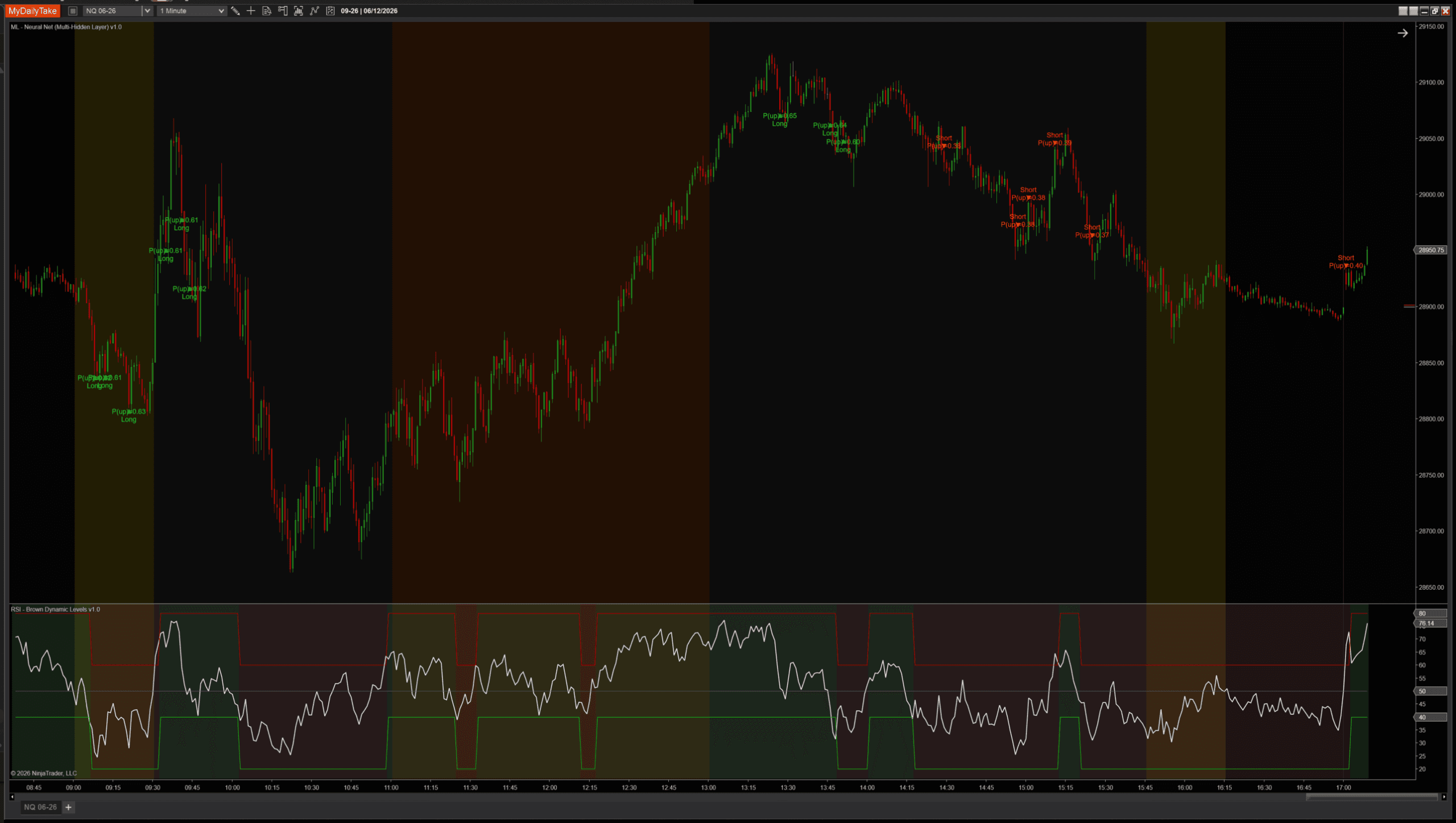
🎚️ Pairing With a Regime Filter
Same defensive pattern as the prior posts: the model can produce contrarian signals during sustained trends, and a simple regime filter vetoes them cheaply. RSI(14) above/below 50 is the simplest version — take longs only when RSI confirms uptrend, take shorts only when it confirms downtrend. Below: a clean run with the regime filter active, the network’s signals aligned with the filter throughout the session:
🛠️ Using It in a Strategy
Everything the indicator computes is exposed as public Series so any strategy can chain off it directly without recomputing the model:
Public Outputs
| Output | Type | Purpose |
|---|---|---|
| ProbabilityUpSeries |
Series | The model's predicted probability of an up move, post-sigmoid output layer. Range [0, 1]. |
| ConfidenceSeries |
Series | |P(up) − 0.5| × 2 — distance from coin-flip, scaled to [0, 1]. 0 = uncertain, 1 = maximum conviction. |
| IsLongSignalSeries |
Series | True on bars where prediction passes the probability gate AND cooldown — long signal fires. |
| IsShortSignalSeries |
Series | True on bars where prediction passes the probability gate AND cooldown — short signal fires. |
Below: a working strategy that combines the network’s signal with an RSI regime filter — long only when the model fires AND RSI confirms uptrend, short only when both confirm downtrend. Same pattern as the prior posts, with the multi-layer Series plugged in:
private MlNeuralNetMultiLayer     nn;
private RSI                       rsi;

protected override void OnStateChange()
{
    if (State == State.SetDefaults)
    {
        Name        = "MhlRsiTrendFollower";
        Calculate   = Calculate.OnBarClose;
    }
    else if (State == State.DataLoaded)
    {
        nn = MlNeuralNetMultiLayer(
            hiddenLayerSizes:       "8, 6",
            hiddenActivation:       MlNeuralNetMultiLayer_Activation.ReLU,
            randomSeed:             42,
            learningRate:           0.005,
            regularizationLambda:   0.0005,
            labelHorizon:           2,
            weightInit:             MlNeuralNetMultiLayer_WeightInitMode.Random,
            labelMode:              MlNeuralNetMultiLayer_LabelMode.CloseToClose,
            minFavorableMoveAtrs:   1.0,
            maPeriod:               8,
            atrPeriod:              50,
            slopeLookback:          2,
            normalizeFeatures:      true,
            normalizationLookback:  200,
            minProbabilityEdge:     0.10,
            signalCooldownBars:     3);

        rsi = RSI(14, 3);
    }
}

protected override void OnBarUpdate()
{
    if (CurrentBar < 300) return;

    // Long: model predicts up AND RSI confirms uptrend regime.
    if (nn.IsLongSignalSeries[0] && rsi[0] > 50)
        EnterLong("NN Long");

    // Short: model predicts down AND RSI confirms downtrend regime.
    if (nn.IsShortSignalSeries[0] && rsi[0] < 50)
        EnterShort("NN Short");
}
Swap RSI for any indicator that exposes a Series — ADX above a threshold, price relative to a higher-timeframe MA, a SuperTrend state. Anything you already trust as a regime tool will compose cleanly.
📝 The Honest Validation Talk (Still)
The same caveat from the prior posts applies, sharper at depth. Every prediction is technically out-of-sample (the training step is one LabelHorizon in arrears), but the model is continuously changing — an “accuracy over the last 1000 bars” figure averages over many different effective models. With 119 parameters on the default depth, the model adapts to recent regime even faster than the shallower siblings, meaning even fewer past bars reflect the model’s current behavior. Walk-forward across multiple regimes is the only honest evaluation, and the work scales with how seriously you want to trust the result.
📦 Download
Install:
- Download the .zip file above.
- In NinjaTrader 8, go to Tools → Import → NinjaScript Add-On.
- Select the downloaded .zip file.
- The indicator will appear under Indicators → indMyDailyTake → ML — Neural Net (Multi-Hidden Layer) v1.0 on your chart.
🎉 Prop Trading Discounts
💥89% off at Bulenox.com with the code MDT89
This is the fourth installment of the Learn NinjaScript ML series. Post 1 covered k-Nearest Neighbors, the memorizing model. Post 2 covered online logistic regression, the simplest compressing model. Post 3 added a single hidden layer — your first “real” neural network. Post 4 (this one) extended depth to any number of layers, and surfaced the practical trade-offs depth brings: vanishing gradients, parameter explosion, and the data hunger that comes with capacity.