ML — Gradient Boosting: The Algorithm Behind XGBoost for NinjaTrader 8
The previous post built a Random Forest — many decision trees, each grown independently on its own slice of the data, their votes averaged. This post keeps the trees but changes how they are built and combined. Gradient boosting grows trees in sequence: each new tree is fitted to the errors the ensemble still makes, and its output is added to a running score. It is the algorithm at the heart of XGBoost — the gradient-boosting library that became a default tool for tabular-data problems — and this post implements its core.
This is the second of the two tree-ensemble posts in the series. Where the forest reduced variance by averaging, boosting reduces error by correction — a different idea, and a model that behaves quite differently on a chart.
🌲 Boosting vs Bagging
The Random Forest used bagging: build many trees independently, in parallel, and average them. No tree knows the others exist. Boosting is the opposite — the trees are built one after another, and each one’s job is defined entirely by the trees before it.
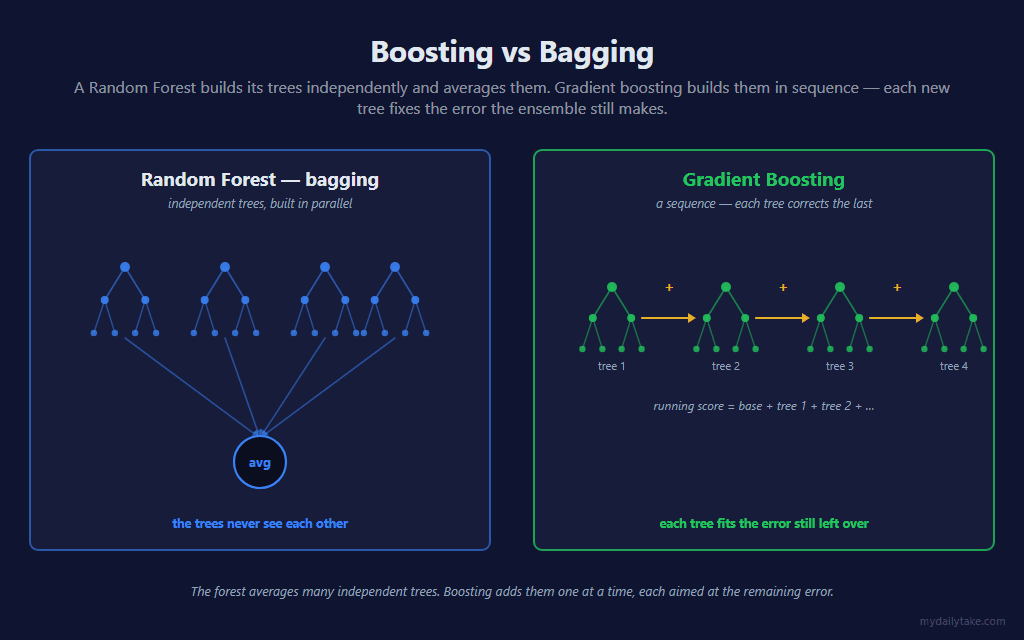
One consequence is worth flagging up front: gradient boosting here is deterministic. There is no bootstrap sample and no random feature subset — the randomness that made the forest work. Given the same training data, boosting always produces the same model. Its diversity comes not from randomness but from the sequence: each tree sees a different problem because it fits what is left over.
🔁 The Boosting Loop
The model works in log-odds space. Every example carries a running score; the predicted probability is the sigmoid of that score. Training is a loop, one tree per round:
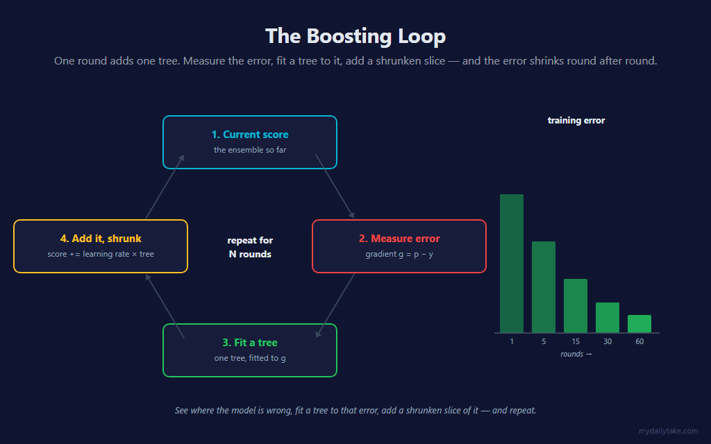
Each round: take the current score for every training example, measure how wrong it is, fit one tree to that error, and add a shrunken slice of the tree back into the score. Repeat. The first tree starts from a flat base score — the log-odds of the training set’s overall up-rate — so the model begins at the right base rate and every tree after that is pure correction:
// Rebuild the whole ensemble. Start from a flat base score, then add NumTrees
// trees one at a time. Before each tree, recompute the gradient and hessian of
// the logistic loss at the current scores; the tree is fitted to those, and its
// (shrunk) output is added back into every example's running score.

private void RebuildEnsemble()
{
    int n = trainCount;

    // Base score — the global log-odds of the training set's up-rate.
    int posCount = 0;
    for (int i = 0; i < n; i++) posCount += trainLabel[i];
    double p0 = (double)posCount / n;
    if (p0 < 0.01) p0 = 0.01;
    if (p0 > 0.99) p0 = 0.99;
    baseScore = Math.Log(p0 / (1.0 - p0));

    for (int i = 0; i < n; i++) scoreBuf[i] = baseScore;

    for (int m = 0; m < NumTrees; m++)
    {
        // Gradient + hessian of the logistic loss at the current scores.
        for (int i = 0; i < n; i++)
        {
            double p = Sigmoid(scoreBuf[i]);
            gradBuf[i] = p - trainLabel[i];
            hessBuf[i] = Math.Max(p * (1.0 - p), 1e-6);
        }

        // Fit tree m to (g, h) over all n examples.
        for (int i = 0; i < n; i++) sampleIdx[i] = i;
        treeNodeCount[m] = 0;
        BuildNode(m, 0, n, 0);

        // Add the new tree's contribution to every example's score.
        for (int i = 0; i < n; i++)
            scoreBuf[i] += PredictTree(m, trainFeat[i]);
    }
}
The phrase “measure how wrong it is” is doing real work. It is not just the sign of the error — boosting uses the gradient and the hessian of the loss, which is what the next section is about.
📐 The Second-Order Step
For the logistic loss, two derivatives describe the error at each example. The gradient g = p − y says how wrong the current prediction is and in which direction. The hessian h = p(1 − p) says how sharply the loss curves there — how confident the prediction is. Classic gradient boosting uses only the gradient; XGBoost uses both, which is what makes it a second-order (Newton) method.
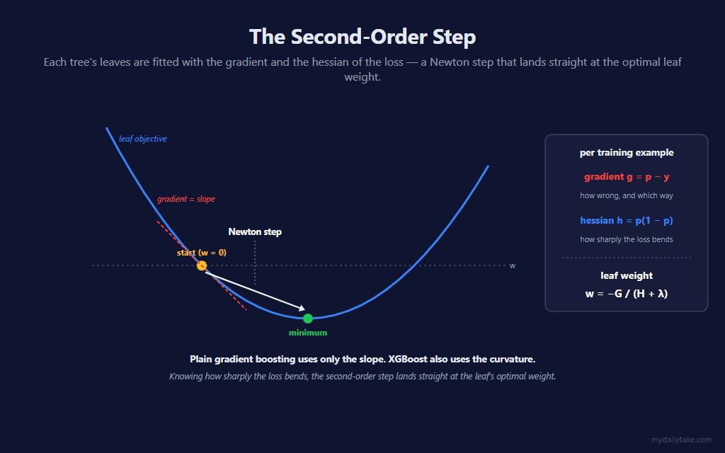
Within a single leaf, the regularized objective is a parabola in the leaf’s weight w: Σ(g·w + ½h·w²) + ½λw². Minimizing it is one step of algebra, and the answer is the leaf’s optimal weight:
w = −G / (H + λ)
where G and H are the sums of the gradients and hessians of the examples that landed in the leaf, and λ is the L2 Lambda regularizer. Because the objective is an exact parabola, the Newton step does not inch toward the minimum — it lands on it in one move. The hessian in the denominator is what makes it a Newton step rather than a plain gradient step.
🌳 Growing a Boosted Tree
Each round’s tree is grown the same recursive way the forest’s trees were — find the best split, partition, recurse — but every node now works with the gradient and hessian sums rather than class counts, and a leaf stores the weight from the formula above (shrunk by the learning rate, for reasons covered shortly):
// Grow one node of a boosted tree. sampleIdx[lo..hi) are the example slots for
// this node; G and H are the sums of their gradients and hessians. The node is
// split in place; it becomes a leaf at the depth cap or when no split has gain.

private int BuildNode(int treeIdx, int lo, int hi, int depth)
{
    GbNode[] tree = trees[treeIdx];
    int nodeIdx   = treeNodeCount[treeIdx]++;

    double G = 0.0, H = 0.0;
    for (int s = lo; s < hi; s++)
    {
        int ex = sampleIdx[s];
        G += gradBuf[ex];
        H += hessBuf[ex];
    }

    int    bestFeat = -1;
    double bestThr  = 0.0;
    int    mid      = lo;
    if (depth < MaxDepth && FindBestSplit(lo, hi, G, H, out bestFeat, out bestThr))
    {
        mid = Partition(lo, hi, bestFeat, bestThr);
        if (mid <= lo || mid >= hi) bestFeat = -1;   // degenerate split — make a leaf
    }

    if (bestFeat < 0)
    {
        // Leaf weight = the regularized optimal Newton step, shrunk by the
        // learning rate:  w = LearningRate * ( -G / (H + lambda) ).
        tree[nodeIdx].Feature    = -1;
        tree[nodeIdx].LeafWeight = LearningRate * (-G / (H + L2Lambda));
        return nodeIdx;
    }

    int left  = BuildNode(treeIdx, lo,  mid, depth + 1);
    int right = BuildNode(treeIdx, mid, hi,  depth + 1);

    tree[nodeIdx].Feature   = bestFeat;
    tree[nodeIdx].Threshold = bestThr;
    tree[nodeIdx].Left      = left;
    tree[nodeIdx].Right     = right;
    return nodeIdx;
}
A node becomes a leaf at the depth cap or when no split is worth taking. Boosted trees are deliberately shallow — the default Max Tree Depth is 3. Each tree is meant to be a weak learner that nudges the score a little; depth and accuracy come from stacking many of them, not from any single deep tree.
✂️ Scoring a Split — the Gain
A split is judged by how much regularized loss it removes. Plugging the optimal leaf weight back into the objective gives each node a score of −½ G²/(H+λ); the gain of a split is the improvement from parent to children, minus a fixed penalty:
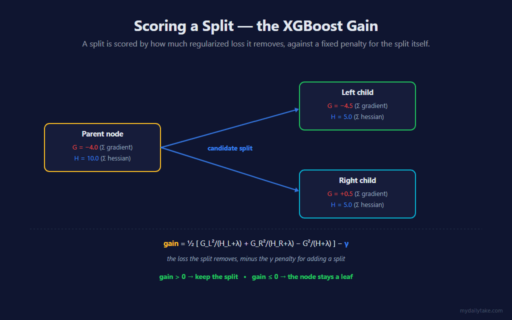
The search sweeps every candidate threshold on every feature — sorting the node’s examples and accumulating the gradient and hessian sums on each side — and keeps the split with the highest gain, provided that gain is positive:
// Score every candidate split across all features by the XGBoost gain and
// return the one with the highest positive gain:
//   gain = ½ [ G_L²/(H_L+λ) + G_R²/(H_R+λ) − G²/(H+λ) ] − γ
// A split must beat the Gamma penalty and leave at least MinChildWeight of
// hessian on each side.

private bool FindBestSplit(int lo, int hi, double G, double H, out int bestFeat, out double bestThr)
{
    bestFeat = -1;
    bestThr  = 0.0;

    int    n          = hi - lo;
    double parentTerm = G * G / (H + L2Lambda);
    double bestGain   = 0.0;   // a split must yield strictly positive gain

    for (int f = 0; f < NumFeatures; f++)
    {
        // sort this node's samples by feature f, carrying their g and h
        for (int s = 0; s < n; s++)
        {
            int ex = sampleIdx[lo + s];
            splitScratch[s].Value = trainFeat[ex][f];
            splitScratch[s].Grad  = gradBuf[ex];
            splitScratch[s].Hess  = hessBuf[ex];
        }
        Array.Sort(splitScratch, 0, n);

        // sweep a threshold between every pair of distinct values
        double GL = 0.0, HL = 0.0;
        for (int i = 0; i < n - 1; i++)
        {
            GL += splitScratch[i].Grad;
            HL += splitScratch[i].Hess;

            if (splitScratch[i].Value == splitScratch[i + 1].Value) continue;

            double GR = G - GL;
            double HR = H - HL;
            if (HL < MinChildWeight || HR < MinChildWeight) continue;

            double gain = 0.5 * (GL * GL / (HL + L2Lambda)
                               + GR * GR / (HR + L2Lambda)
                               - parentTerm) - Gamma;

            if (gain > bestGain)
            {
                bestGain = gain;
                bestFeat = f;
                bestThr  = 0.5 * (splitScratch[i].Value + splitScratch[i + 1].Value);
            }
        }
    }

    return bestFeat >= 0;
}

// Rearrange sampleIdx[lo..hi) so examples with feature[feat] <= thr come first;
// the returned index is the start of the right child.

private int Partition(int lo, int hi, int feat, double thr)
{
    int mid = lo;
    for (int s = lo; s < hi; s++)
    {
        if (trainFeat[sampleIdx[s]][feat] <= thr)
        {
            int tmp = sampleIdx[mid];
            sampleIdx[mid] = sampleIdx[s];
            sampleIdx[s]   = tmp;
            mid++;
        }
    }
    return mid;
}
Two regularizers live in this search. Gamma is subtracted directly from every gain — a split must clear that bar or it is not made, which prunes weak splits. Min Child Weight requires each side of a split to hold a minimum total hessian, so the model cannot carve a leaf out of a few low-confidence examples. Both push the trees toward simpler, steadier shapes.
🪜 Shrinkage — the Learning Rate
If each tree applied its full Newton step, the second tree would spend its effort undoing the first’s overshoot. So every tree’s contribution is scaled down by the learning rate before it is added — XGBoost calls this shrinkage.
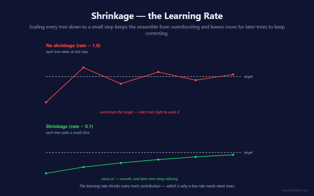
Small steps mean each tree is a gentle correction, and later trees always have useful work left to do. The trade-off is direct: a lower Learning Rate generalizes better but needs more trees to get there. The default pairs a rate of 0.10 with 60 rounds — and the chart section below shows what happens when you change the tree count.
🔮 Making a Prediction
Prediction is the sum the loop was building all along. The current bar’s features run down every tree; each tree returns its leaf weight; those weights are added to the base score, and the sigmoid turns the total into a probability:
// The ensemble score is the base score plus every tree's leaf weight; the
// probability is the sigmoid of that score.

private double EnsemblePredict(double[] feat)
{
    double score = baseScore;
    for (int m = 0; m < NumTrees; m++) score += PredictTree(m, feat);
    return Sigmoid(score);
}

// Walk one tree from the root: at each internal node go left if the feature is
// at or below the threshold, else right. The leaf's stored weight is this
// tree's (shrunk) contribution to the log-odds score.

private double PredictTree(int t, double[] feat)
{
    GbNode[] tree = trees[t];
    int idx = 0;
    while (tree[idx].Feature >= 0)
        idx = feat[tree[idx].Feature] <= tree[idx].Threshold ? tree[idx].Left : tree[idx].Right;
    return tree[idx].LeafWeight;
}
🔄 Batch Retraining
Like the Random Forest, a boosted ensemble is a batch learner. The trees are a fixed structure built in a specific sequence; there is no way to fold in one new bar without rebuilding. So the indicator keeps a rolling Training Window of the most recent look-ahead-safe (features, label) examples — each bar’s features from Label Horizon ago, paired with the now-observable realized direction — and every Retrain Interval bars it rebuilds the whole ensemble from scratch. The model is fixed between rebuilds and steps to a new ensemble at each retrain.
📊 What This Looks Like on a Chart
Same indicator, same NQ session. Only the number of boosting rounds changes — and unlike the forest’s depth knob, this one moves the chart a lot. Start with the default:
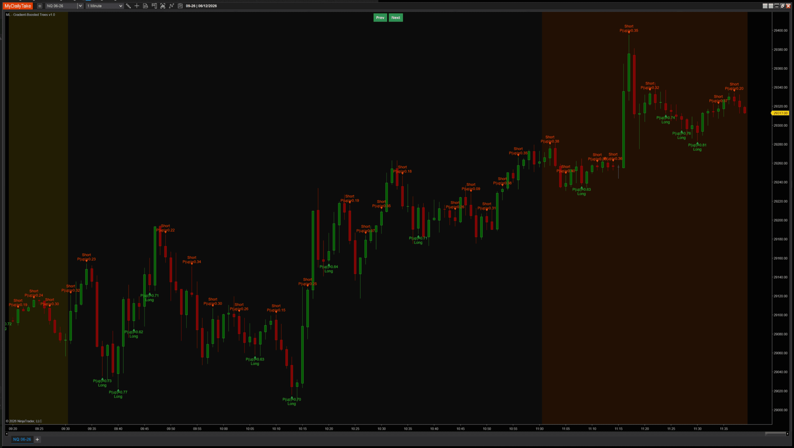
Default settings (60 trees). A moderate, confident signal set.
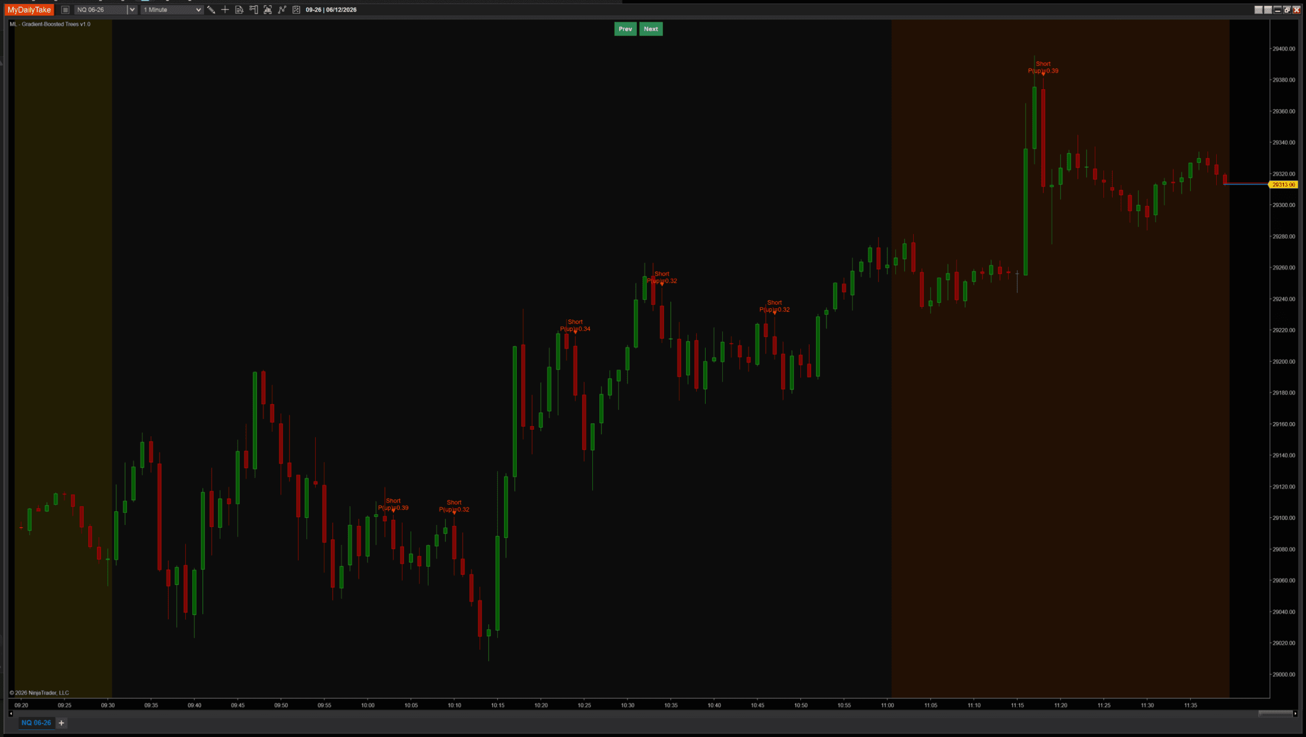
5 trees. Barely-boosted — almost nothing fires.
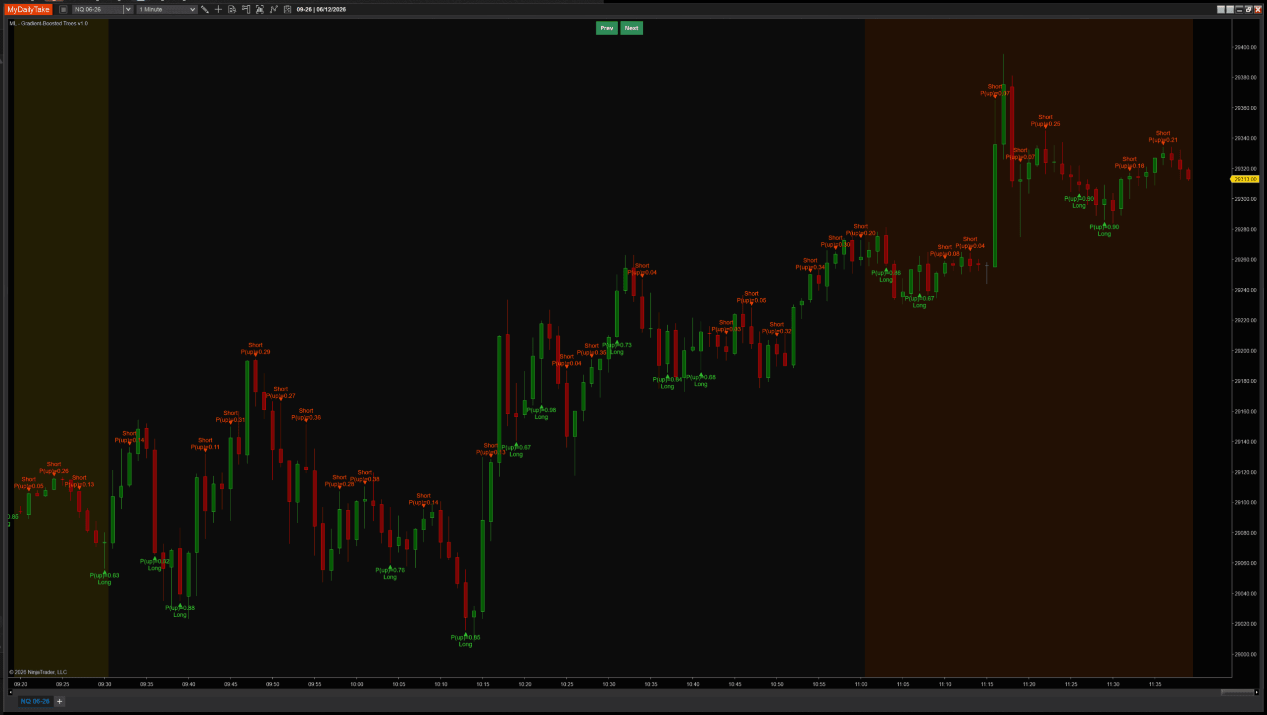
300 trees. Heavily boosted — dense signals and very extreme probabilities.
This is the boosting story in three frames. With only 5 trees the ensemble has added five small corrections to the base score — it has barely moved off the base rate, so P(up) stays near 0.5 and almost nothing clears the Min Probability Edge gate. The default 60 rounds produce a confident, working signal set. At 300 rounds the model is pushing probabilities to 0.04 and 0.98 — and that is worth reading as a warning, not a triumph. Directional prediction from three features is close to a coin flip; a model that claims 98% certainty has almost certainly fitted noise. This is overfitting made visible, and it is exactly why the regularizers — Learning Rate, L2 Lambda, Gamma, Min Child Weight — exist. More rounds is not more skill.
⚙️ Settings
The indicator’s settings are grouped into five categories. Boosting holds the gradient-boosting hyperparameters. Learning controls the training buffer, the retrain cadence, and the labeling. Features controls what the model sees. Signal controls when triangles fire. Display is cosmetic-only.
Boosting
| Parameter | Description |
|---|---|
| Number of Trees | Number of boosting rounds — one tree is added per round. Each new tree corrects the errors the current ensemble still makes. More trees fit the training data more closely; paired with a small Learning Rate, more rounds generalize better at the cost of compute. Default 60. |
| Max Tree Depth | Maximum depth of each boosted tree. Gradient boosting works best with shallow trees — weak learners — and many of them. Depth 2 to 4 is typical; the default is 3. |
| Learning Rate | Shrinkage applied to every tree's contribution (XGBoost's 'eta'). A small rate makes each tree a gentle correction so later trees can keep refining the fit. Lower rate = needs more trees but generalizes better. Default 0.10. |
| Min Child Weight | Minimum total hessian a split's child node must hold. The hessian of the logistic loss measures prediction confidence, so this stops the model from carving leaves out of a few uncertain samples. Higher = more conservative. Default 1.0. |
| L2 Lambda | L2 regularization on the leaf weights (XGBoost's 'lambda'). It appears in the denominator of both the leaf-weight and split-gain formulas, shrinking leaf values toward zero and damping over-confident trees. Default 1.0. |
| Gamma (min split gain) | Minimum loss reduction required to make a split (XGBoost's 'gamma'). A split is only kept if its gain exceeds this penalty, so larger values prune weak splits and grow simpler trees. Default 0.0. |
Learning
| Parameter | Description |
|---|---|
| Training Window (bars) | Number of recent look-ahead-safe (feature, label) examples kept for training. Each ensemble rebuild is fitted to this rolling window, so older examples fall out over time. Default 300. |
| Retrain Interval (bars) | How often the whole ensemble is rebuilt. A boosted ensemble cannot be updated one bar at a time, so the model retrains in batches every N bars from the current Training Window. Smaller = more responsive but more compute. Default 25. |
| Label Horizon (bars) | How many bars ahead the realized direction is observed. Each bar contributes one training example using the features from N bars ago, whose forward outcome is now known — this keeps training look-ahead-safe. |
| Label Mode | How the training label is defined. CloseToClose: y = 1 if Close at the end of the Label Horizon window is above Close at the training bar. FavorableExcursion: y = 1 if the long-side favorable move beat the short-side move during the window (uses bar highs/lows); bars below Min Favorable Move are skipped as chop. |
| Min Favorable Move (ATRs) | ONLY USED WHEN Label Mode = FavorableExcursion. Minimum favorable excursion (in ATRs at entry) required during the post-bar window for the bar to become a training example. |
Features
| Parameter | Description |
|---|---|
| MA Period | Period of the moving average used in the distance-from-MA feature, and the smoothing window for the ATR regime-ratio feature. |
| ATR Period | Period of the ATR used to scale every feature into volatility units, so distance comparisons stay consistent across regimes. |
| Slope Lookback (bars) | Number of bars over which the slope feature is measured: (Close[0] − Close[N]) / ATR. |
| Normalize Features (Z-Score) | Master toggle for z-score normalization. Boosted trees are scale-invariant to fixed transforms, but the rolling z-score still helps by making each feature stationary against its own recent distribution. Recommended ON for parity with the rest of the series. |
| Normalization Lookback (bars) | Window used to compute the rolling mean and standard deviation that z-score the features. Each bar uses its own local-time stats. |
Signal
| Parameter | Description |
|---|---|
| Min Probability Edge | How far the ensemble's predicted probability of an up move must be from 0.5 before a signal fires. 0.10 means a long fires when P(up) > 0.60 and a short fires when P(up) < 0.40. |
| Signal Cooldown (bars) | Minimum number of bars between consecutive signals. Higher values space signals out so the chart stays readable. |
Display
| Parameter | Description |
|---|---|
| Marker Offset (ticks) | Vertical offset of the signal triangle from the bar's high (shorts) or low (longs), in ticks. |
| Label Offset (ticks) | Distance from the bar to the text label, in ticks. Should be larger than Marker Offset so the label sits beyond the triangle. |
| Show Labels | Render the predicted-probability label beside each signal triangle. |
| Label Font Size | Font size for the signal labels. |
The honest way to tune these is in pairs: drop the Learning Rate and raise Number of Trees together, and lean on L2 Lambda and Gamma if the signals look as over-confident as the 300-tree chart above.
🎚️ Pairing With a Regime Filter
Same defensive pattern as the prior posts. An RSI(14) above or below 50 vetoes counter-trend signals, so the model is only allowed to fire with the broader trend:
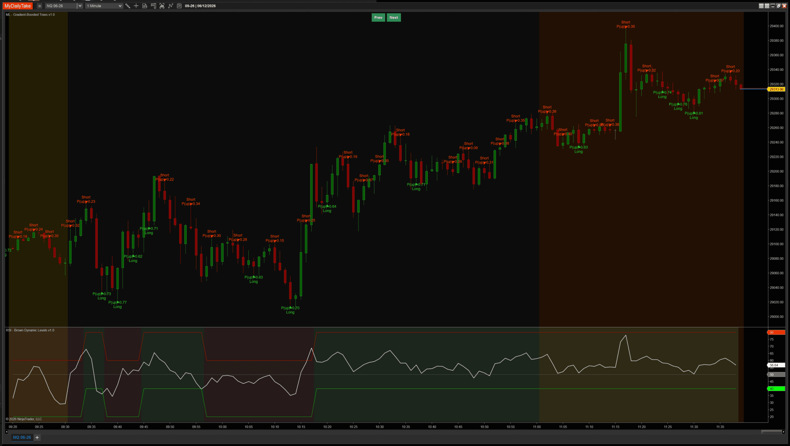
The boosted model’s raw output is a probability; the regime filter is a separate, far simpler model. Combining a learned signal with a transparent rule-based veto is a dependable way to keep the model from fighting the obvious trend.
🛠️ Using It in a Strategy
The indicator exposes its outputs as public Series so a strategy can consume the model directly:
Public Outputs
| Output | Type | Purpose |
|---|---|---|
| ProbabilityUpSeries |
Series | The ensemble's predicted probability of an up move — the sigmoid of the boosted score. Range [0, 1]. |
| ConfidenceSeries |
Series | |P(up) − 0.5| × 2 — distance from a coin-flip, scaled to [0, 1]. 0 = uncertain, 1 = maximum conviction. |
| IsLongSignalSeries |
Series | True on bars where the prediction passes the probability gate AND the cooldown — a long signal fires. |
| IsShortSignalSeries |
Series | True on bars where the prediction passes the probability gate AND the cooldown — a short signal fires. |
Below is a working strategy that combines the boosted model’s signal with the RSI regime filter from the previous section — a long is allowed only when the model predicts up and RSI is above 50, and the mirror for shorts:
private MlGradientBoost      nn;
private RSI                  rsi;

protected override void OnStateChange()
{
    if (State == State.SetDefaults)
    {
        Name        = "GradientBoostRsiTrendFollower";
        Calculate   = Calculate.OnBarClose;
    }
    else if (State == State.DataLoaded)
    {
        nn = MlGradientBoost(
            numTrees:               60,
            maxDepth:               3,
            learningRate:           0.10,
            minChildWeight:         1.0,
            l2Lambda:               1.0,
            gamma:                  0.0,
            trainingWindow:         300,
            retrainInterval:        25,
            labelHorizon:           2,
            labelMode:              MlGradientBoost_LabelMode.CloseToClose,
            minFavorableMoveAtrs:   1.0,
            maPeriod:               8,
            atrPeriod:              50,
            slopeLookback:          2,
            normalizeFeatures:      true,
            normalizationLookback:  200,
            minProbabilityEdge:     0.10,
            signalCooldownBars:     3);

        rsi = RSI(14, 3);
    }
}

protected override void OnBarUpdate()
{
    // The indicator gates its own signals through warmup; this is a safety margin.
    if (CurrentBar < 400) return;

    // Long: the boosted model predicts up AND RSI confirms the uptrend regime.
    if (nn.IsLongSignalSeries[0] && rsi[0] > 50)
        EnterLong("GB Long");

    // Short: the boosted model predicts down AND RSI confirms the downtrend regime.
    if (nn.IsShortSignalSeries[0] && rsi[0] < 50)
        EnterShort("GB Short");
}
📝 The Honest Validation Talk (Still)
Gradient boosting is, on most tabular problems, the strongest model in this series — which makes it the most dangerous one to trust without checking. It will fit a training window extremely well, and the 300-tree chart is a reminder of how confidently it will do so even when the signal is not there. It also shares the Random Forest’s quiet trap: it retrains in batches, so its behavior steps from one ensemble to the next, and “accuracy over the last N bars” averages over several different models. None of that is a reason to avoid it. It is a reason to evaluate it honestly — walk-forward across multiple regimes is still the only honest test, and the work scales with how seriously you intend to trust the result.
📦 Download
Install:
- Download the .zip file above.
- In NinjaTrader 8, go to Tools → Import → NinjaScript Add-On.
- Select the downloaded .zip file.
- The indicator will appear under Indicators → indMyDailyTake → ML – Gradient-Boosted Trees v1.0 on your chart.


This is the ninth installment of the Learn NinjaScript ML series. Posts 1–7 built the neural-network thread — k-Nearest Neighbors, online logistic regression, a single hidden layer, configurable depth, the Adam optimizer, a recurrent network, and the LSTM. Post 8 turned to tree ensembles with the Random Forest. Post 9 (this one) builds gradient-boosted trees — the algorithm behind XGBoost. Post 10 closes the series with walk-forward validation: how to actually test any of these.