ML — Single-Hidden-Layer Neural Network: Your First Multi-Layer Net for NinjaTrader 8
The prior post built a single-neuron model — three weights, a bias, and a sigmoid that turned a weighted sum into P(up). It worked, but its limits were architectural: a single neuron can only carve the feature space with a straight line. Any pattern that requires the features to interact non-linearly — “high distFromMa AND positive slope means continuation, but high distFromMa AND negative slope means reversal” — is invisible to a one-neuron model.
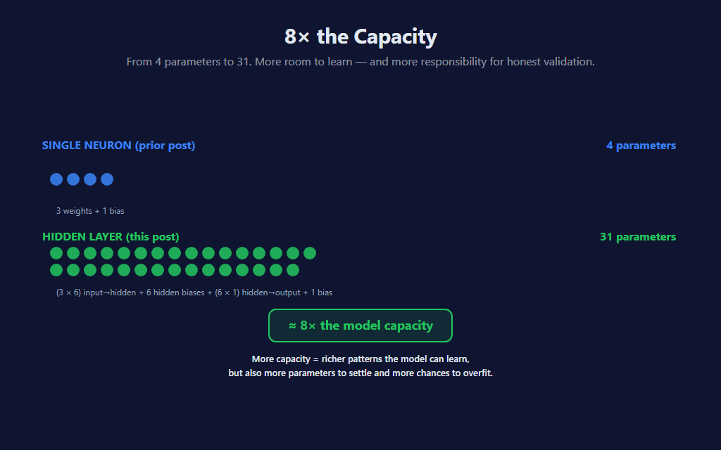
This post adds a hidden layer. The architecture goes from 3 inputs → 1 sigmoid output to 3 inputs → 6 hidden neurons (with their own activation) → 1 sigmoid output. Parameter count goes from 4 to 31. The training algorithm goes from one chain-rule step to two — the famous “backpropagation” you’ve heard about. And the model picks up the ability to learn the non-linear feature interactions a single neuron cannot represent.
🧠 What a Hidden Layer Actually Adds
The single-neuron model from the prior post is, in mathematical terms, a linear classifier. Its decision boundary — the set of feature combinations where P(up) = 0.5 — is a hyperplane. In feature space, that’s a flat line slicing through the data. Anything that needs a curve to separate — a circle, a corner, a region in the middle of the cloud — is fundamentally beyond it.
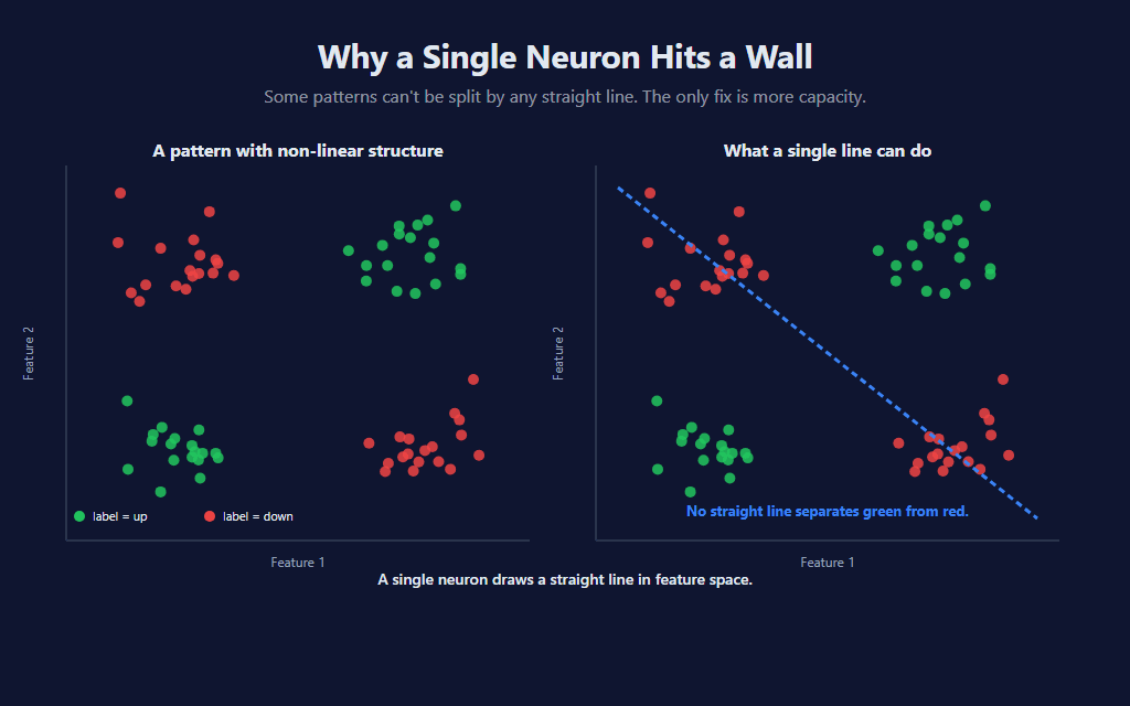
The diagonal-pair pattern above is the canonical example of why a linear model isn’t enough. No straight line separates the green outcomes from the red ones — they live in opposite corners, not opposite halves of the plane. A single neuron can’t represent this. A model with even one hidden layer can, because the hidden neurons can each learn to recognize a different region of the input space, and the output layer combines those regions into the final prediction.
That’s what “capacity” means in neural-network speak. More neurons = more flexibility to fit complex shapes. Whether that flexibility helps or hurts depends on whether the underlying data actually has those shapes — which is the central trade-off we’ll come back to at the end.
🏗️ The Architecture: 3 → 6 → 1
Three input features (the same trend-following triplet from the prior post — distFromMa, slope, atrRegime), six hidden neurons, one sigmoid output. The hidden neurons each receive all three inputs through their own learned weights, run the result through an activation function (default tanh), and forward their output to the single output neuron, which combines them into the final probability.
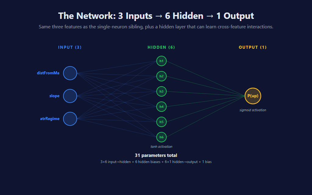
The parameter count tells the story of the capacity jump. The prior single-neuron model had 4 numbers to learn: 3 weights and a bias. This network has 31: 18 hidden weights (3 inputs × 6 hidden neurons) + 6 hidden biases + 6 output weights + 1 output bias. About 8× more knobs to tune.
Six hidden neurons isn’t magic — it’s a starting heuristic of roughly twice the input count for shallow networks on small-feature problems. Bump up if you suspect your data has rich feature interactions; bump down if signals look noisy on limited data. The HiddenNeurons property is the first knob to tune.
🎚️ Choosing the Hidden Activation
The output layer is always a sigmoid because we want a probability in [0, 1]. The hidden layer is more flexible — three reasonable choices, each with a different shape and different gradient behavior:
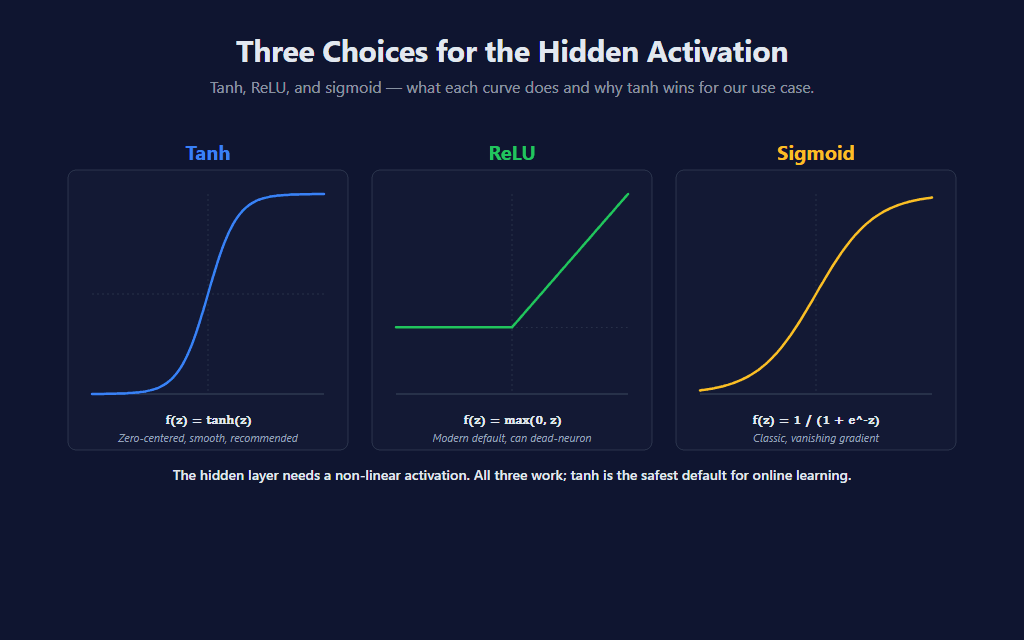
- Tanh (default, recommended): zero-centered S-curve, smooth derivative, the historical default for shallow networks. Stable under online single-step gradient descent.
- ReLU: the modern default for deep networks because its gradient doesn’t saturate at high inputs. The drawback under online learning is “dead neurons” — if a neuron’s pre-activation goes negative early and the gradient never pushes it back, that neuron emits zero forever and contributes nothing to predictions or updates.
- Sigmoid: the classic choice but suffers from vanishing gradient at extreme inputs (the curve flattens, derivatives approach zero, and updates effectively stall on neurons that have saturated).
For a single hidden layer of six neurons trained one bar at a time, all three work — the network is shallow enough that none of the failure modes are catastrophic. Tanh’s symmetry around zero pairs cleanest with the z-score-normalized features (which are also zero-centered), and that’s why it’s the default. The HiddenActivation dropdown lets you switch.
➡️ The Forward Pass
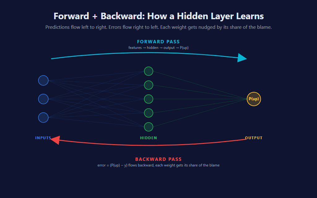
The forward pass is exactly what the architecture diagram shows, written in code. For each hidden neuron, dot-product the inputs with the neuron’s weights, add the bias, run through the activation. Then dot-product the hidden activations with the output weights, add the output bias, sigmoid for the final probability. Two layers, two matrix operations.
// Forward pass — runs every bar to compute P(up).
// inputs[NumFeatures] -> hiddenPre[HiddenNeurons] -> hiddenAct[HiddenNeurons]
// -> output -> sigmoid -> P(up).
// Caches hiddenPre and hiddenAct on instance fields so the backward pass can
// reuse them without recomputing.

private double ForwardPass(double[] inputs)
{
    // Hidden layer: pre-activation = Wh . inputs + bh, then activation.
    for (int h = 0; h < HiddenNeurons; h++)
    {
        double z = bh[h];
        for (int i = 0; i < NumFeatures; i++)
            z += Wh[h][i] * inputs[i];
        hiddenPre[h] = z;
        hiddenAct[h] = Activate(z);
    }

    // Output layer: zOut = Wo . hiddenAct + bo, then sigmoid.
    double zOut = bo;
    for (int h = 0; h < HiddenNeurons; h++)
        zOut += Wo[h] * hiddenAct[h];

    return Sigmoid(zOut);
}
The cached hiddenPre and hiddenAct arrays aren’t required for the prediction — the function could just compute and return. They exist because the backward pass (next section) will need to know exactly what each hidden neuron output during this forward pass, and recomputing them would be wasted work. This is a standard optimization in any neural-network implementation: forward-pass intermediates are stashed and reused during backprop.
⬅️ Backpropagation, in Plain English
Backpropagation is the step that intimidates people new to neural nets, but the idea is simpler than its reputation. Once we have a prediction p and a label y, we know the prediction was wrong by some amount. The question backprop answers is: which weights, in which layer, contributed to that error, and by how much? Once we know that, we nudge each weight in proportion to its contribution.
The trick is the chain rule. The error at the output is a function of the output weights AND the hidden activations AND the hidden weights AND the inputs. The chain rule from calculus lets us decompose that long chain of dependencies into a product of simpler local derivatives — one for each layer — and propagate the error backward through the network step by step. Each layer’s gradient depends on the gradient flowing in from the layer ahead of it (which is why we go backward from the output).
Two pieces of math make this manageable in code:
- The cross-entropy loss combined with a sigmoid output collapses the output-layer gradient to
error = pTrain − y. No messy derivative — just the prediction minus the label. The same simplification that made the prior post’s update step a one-liner. - The gradient flowing back into hidden neuron
hiserror × Wo[h]— the output weight scales how much that hidden neuron contributed to the final prediction. Multiply by the activation’s derivative at that neuron’s pre-activation value, and you have the local gradient for that neuron’s pre-activation.
// Backprop — chain-rule gradient descent through both layers.
// Cross-entropy loss with sigmoid output simplifies the output-layer gradient
// to error = pTrain - y. The gradient at hiddenAct[h] flows back as error * Wo[h]
// (we use the OLD Wo[h] before the output-layer update, which the loop preserves).

private void Backprop(double[] inputs, double pTrain, double y)
{
    double error = pTrain - y;   // dL/dzOut for cross-entropy + sigmoid

    for (int h = 0; h < HiddenNeurons; h++)
    {
        // Gradient flowing into hidden neuron h from the output side.
        double dHiddenAct = error * Wo[h];
        double dHiddenPre = dHiddenAct * ActivationDerivative(hiddenPre[h], hiddenAct[h]);

        // Hidden-layer weight updates: dL/dWh[h][i] = dHiddenPre * inputs[i].
        for (int i = 0; i < NumFeatures; i++)
        {
            double grad = dHiddenPre * inputs[i] + RegularizationLambda * Wh[h][i];
            Wh[h][i] -= LearningRate * grad;
        }
        bh[h] -= LearningRate * dHiddenPre;

        // Output-layer weight update for this hidden -> output edge.
        double gradWo = error * hiddenAct[h] + RegularizationLambda * Wo[h];
        Wo[h] -= LearningRate * gradWo;
    }

    bo -= LearningRate * error;
}
The order matters. Inside the loop, we compute dHiddenAct = error × Wo[h] using the old output weight, then update the hidden weights, then update the output weight. If we updated Wo[h] first, the back-propagation calculation would use the new weight and the gradients for the hidden layer would be subtly wrong. Read the loop body carefully — the four-line dance (compute back-prop signal, update hidden weights, update hidden bias, update output weight) is the structural heart of every neural-network library, just written without the abstraction.
⚖️ Two Ways to Label a Bar (Same as Before)
The label rule that defines what “correct” means is the same parameter from the prior post — LabelMode — and the trade-off between the two modes hasn’t changed. Restating briefly:
- CloseToClose:
y = 1ifClose[0] > Close[trainBar]. Tracks pure close-to-close direction. Trains on every observable bar. - FavorableExcursion:
y = 1if the maximum favorable excursion in the LONG direction beat the SHORT direction during the LabelHorizon window. Skips bars belowMinFavorableMoveAtrs— chop bars don’t train.
The choice of label still defines what the model is trying to predict, and that choice still matters more than the architecture. A 31-parameter neural network with a poorly-chosen label rule is worse than a 4-parameter linear model with a thoughtful one. Capacity does not rescue you from labeling the wrong target.
🔁 The Update Step
The update logic hasn’t changed structurally from the prior post. Compute the label using the bar from LabelHorizon ago (whose forward outcome is now observable), do a forward pass at that bar with the current weights, run one step of backprop. The only difference is that “one step of backprop” now means propagating the error through two layers instead of one.
// Update step — runs every bar (when training conditions are met).
// Uses the bar from LabelHorizon ago, whose forward outcome is now observable.
int trainBar = LabelHorizon;
bool   trainThisBar = false;
double y            = 0.0;

if (LabelMode == MlNeuralNetSingleHidden_LabelMode.CloseToClose)
{
    y = Close[0] > Close[trainBar] ? 1.0 : 0.0;
    trainThisBar = true;
}
else // FavorableExcursion: y = 1 if MFE_long > MFE_short during the window.
{
    double closeAtTrain = Close[trainBar];
    double safeAtrTrain = atr[trainBar] > 1e-9 ? atr[trainBar] : TickSize;

    double maxHigh = double.MinValue;
    double minLow  = double.MaxValue;
    for (int b = 0; b < LabelHorizon; b++)
    {
        if (High[b] > maxHigh) maxHigh = High[b];
        if (Low[b]  < minLow)  minLow  = Low[b];
    }

    double mfeLong  = (maxHigh    - closeAtTrain) / safeAtrTrain;
    double mfeShort = (closeAtTrain - minLow)     / safeAtrTrain;

    if (Math.Max(mfeLong, mfeShort) >= MinFavorableMoveAtrs)
    {
        y = mfeLong > mfeShort ? 1.0 : 0.0;
        trainThisBar = true;
    }
}

if (trainThisBar)
{
    GetFeaturesInto(scratchRaw, trainBar);
    NormalizeInto(scratchNorm, scratchRaw, trainBar);

    // Forward pass at trainBar with current weights, then one backprop step.
    double pTrain = ForwardPass(scratchNorm);
    Backprop(scratchNorm, pTrain, y);
}
Look-ahead safety is preserved by the same mechanism: the prediction the user sees on bar zero uses weights that were last updated using a bar from LabelHorizon ago — so the model has never seen the future. The training step is one bar in arrears by construction, and the prediction is fully causal.
📐 What the Decision Boundary Looks Like Now
The single-neuron model could only carve feature space with a straight line. The hidden-layer model can carve it with curves, corners, and disjoint regions. Same data, same features — what’s reachable is fundamentally different:
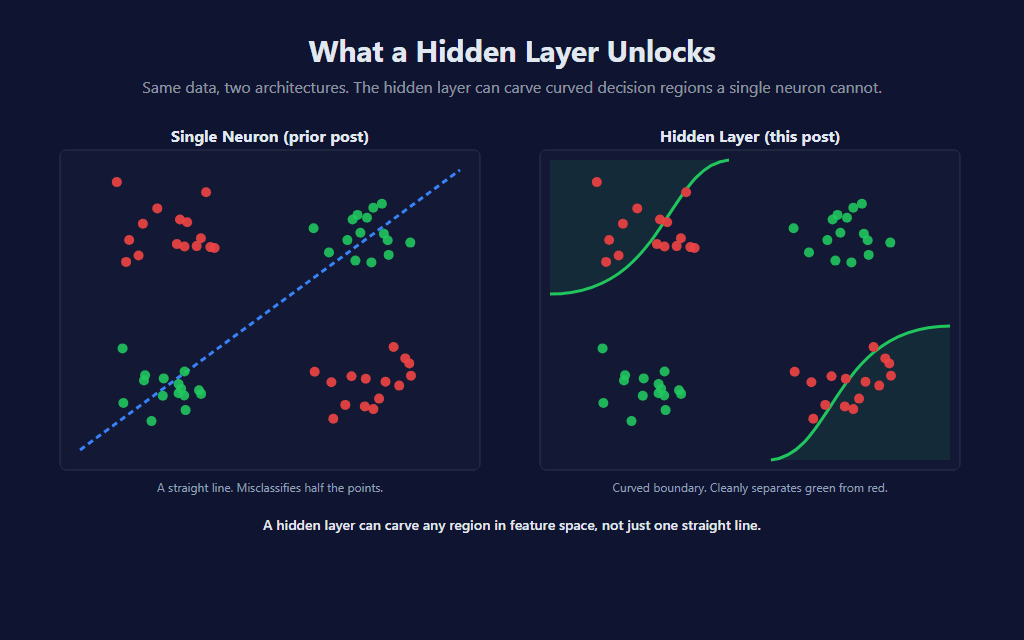
This is the architectural promise made literal. The hidden layer learns a set of intermediate features — combinations of the raw inputs that the output layer then combines linearly. With six hidden neurons, the model can in principle represent any sufficiently smooth decision surface that a much larger network can. With our three input features and the small online-update steps, what it actually learns is a softer version of that — small curvatures rather than sharp corners.
💪 Where the Hidden Layer Helps, and Where It Doesn’t
The hidden layer fixes one specific problem from the prior post: it can represent non-linear feature interactions. If the underlying market dynamic is “extreme distFromMa AND positive slope continues, but extreme distFromMa AND negative slope reverts,” the hidden layer can learn that. The single-neuron model could not.
Two things the hidden layer doesn’t fix:
Mean-reversion bias still applies. The bias-toward-mean-reversion-during-trends behavior from the prior post isn’t a property of the architecture — it’s a property of the dataset. Across a typical mix of regimes, bars with extreme distFromMa or slope often revert more than they continue. A model with more capacity learns the same pattern, sometimes more sharply. During a sustained directional trend the network can still produce contrarian signals at extremes, the same way the single neuron did. Pairing with a regime filter (next section) is still the right defensive step.
More capacity = more risk of overfitting. Thirty-one parameters is comfortable for the kind of tick-by-tick training data a chart provides — there’s plenty of effective sample size in a typical session. But the door is now open, and bumping HiddenNeurons well beyond 6 or weakening the L2 regularization will start producing signals that look great on the bar they were trained on and don’t generalize. The defaults — 6 hidden neurons, regularization 0.0001 — are deliberately on the conservative side.
🛠️ Building the Indicator — Default Setup
Default settings on NQ 1-minute showing the network firing high-conviction signals during a sustained morning rally:
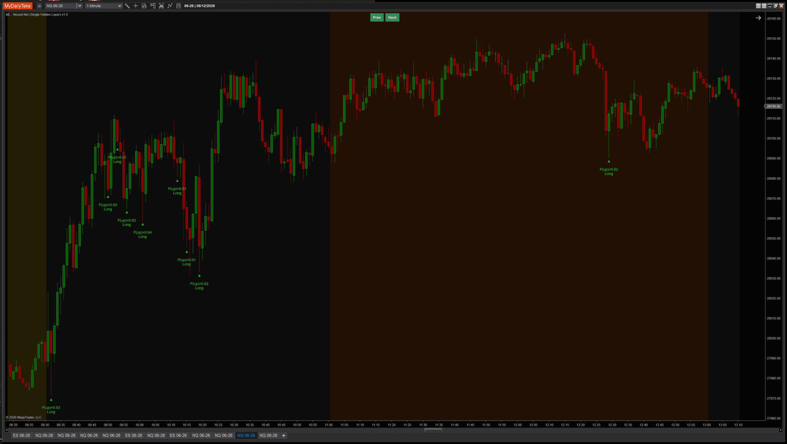
Visual language matches the prior two ML posts: green TriangleUp markers below long-signal bars, red TriangleDown markers above shorts, plus a two-line label showing the predicted P(up) and direction. All three indicators (k-NN, single-neuron, single-hidden-layer) read consistently when stacked on the same chart.
⚙️ Settings
The indicator’s settings are grouped into five categories. Architecture picks the network’s shape and reproducibility seed. Learning controls how the model adapts. Features controls what the model sees. Signal controls when triangles fire. Display is cosmetic-only.
Architecture
| Parameter | Description |
|---|---|
| Hidden Neurons | Number of neurons in the hidden layer. 6 (= 2 × input features) is the conventional starting point for shallow networks. Bump up for richer feature interactions; bump down if signals look noisy on small datasets. With 3 inputs and 6 hidden neurons, total parameter count is 31 — about 8× the 4 parameters of the prior post's single-neuron model. |
| Hidden Activation | Activation function on the hidden layer. Tanh: zero-centered, smooth, the safest default for online learning — recommended. ReLU: modern default for deep nets but can suffer from "dead neuron" failure under online single-step gradient descent if a neuron's pre-activation goes negative early and never recovers. Sigmoid: classic but suffers from vanishing-gradient at extreme inputs. |
| Random Seed | Seed for the random weight initialization (when Weight Init = Random). Same seed produces the same starting weights — useful for reproducible testing or comparing different architectures fairly. Change to explore whether the model converges differently from a different starting point. Has no effect when Weight Init = Zero. |
Learning
| Parameter | Description |
|---|---|
| Learning Rate | Step size for each weight update. Larger = adapts faster but jitters; smaller = smoother but slower to react. With more parameters than the single-neuron sibling (31 vs 4), slightly smaller values (0.005-0.01) often produce more stable training. |
| Regularization Lambda (L2) | L2 penalty that pulls weights gently toward zero each update so they don't drift to extreme values when a feature is noisy. With more parameters, regularization matters more — recommended 0.0001 to 0.001. 0 disables regularization. |
| Label Horizon (bars) | How many bars ahead the realized direction is observed. The model updates each bar using the feature vector from N bars ago, whose forward direction is now known — this is what makes the training step look-ahead-safe. |
| Weight Init | Zero starts every weight at 0 — but ALL hidden neurons would learn identical weights (the symmetry-breaking problem). Strongly recommend Random for multi-neuron networks. Random uses activation-aware scaling: He scaling for ReLU, Xavier/Glorot for tanh and sigmoid, so initial pre-activations stay in the responsive range of each function. |
| Label Mode | How the training label is defined. CloseToClose: y = 1 if Close at end of LabelHorizon window is above Close at trainBar. FavorableExcursion: y = 1 if max favorable excursion in the LONG direction beat the SHORT direction during the window — uses bar highs/lows so wicks count, and skips bars below Min Favorable Move (chop). The choice fundamentally shapes the model's character. |
| Min Favorable Move (ATRs) | ONLY USED WHEN Label Mode = FavorableExcursion. Minimum favorable excursion (in ATRs at entry) required during the post-bar window for the model to update. Below this threshold, the bar's follow-on was just chop — we skip the weight update. Set to 0 to train on every observable bar. |
Features
| Parameter | Description |
|---|---|
| MA Period | Period of the moving average used in the distFromMa feature, and used as the smoothing window for the ATR regime ratio. Smaller = more reactive; larger = trend-anchored. |
| ATR Period | Period of the ATR used to scale every feature into volatility units, so distance comparisons stay consistent across regimes. |
| Slope Lookback (bars) | Number of bars over which the slope feature is measured: (Close[0] − Close[N]) / ATR. Smaller = momentum thrust; larger = trend persistence. |
| Normalize Features (Z-Score) | Master toggle for z-score normalization. When ON, each feature is rescaled against its own historical rolling stats so a 1-σ extreme reading means the same thing across regimes. Recommended ON. |
| Normalization Lookback (bars) | Window used to compute the rolling mean / stddev that z-score the features. Each bar uses its own local-time stats — a 2008 bar against 2008's distribution, a 2024 bar against 2024's. |
Signal
| Parameter | Description |
|---|---|
| Min Probability Edge | How far the predicted probability of an up move must be from 0.5 before a signal fires. 0.10 means: long fires when P(up) > 0.60, short fires when P(up) < 0.40. Larger values produce fewer, higher-conviction signals. |
| Signal Cooldown (bars) | Minimum bars between consecutive signals. Higher values space signals out so the chart stays readable; lower values let signals come in clusters during sustained moves. Set to 0 to fire on every qualifying bar. |
Display
| Parameter | Description |
|---|---|
| Marker Offset (ticks) | Vertical offset of the signal triangle from the bar's high (shorts) / low (longs), in ticks. |
| Label Offset (ticks) | Distance from the bar to the text label, in ticks. Should be larger than Marker Offset so the label sits beyond the triangle. |
| Show Labels | Render the predicted-probability label beside each signal triangle. Turn off for a marker-only chart. |
| Label Font Size | Font size for the signal labels. |
🎚️ Pairing With a Regime Filter
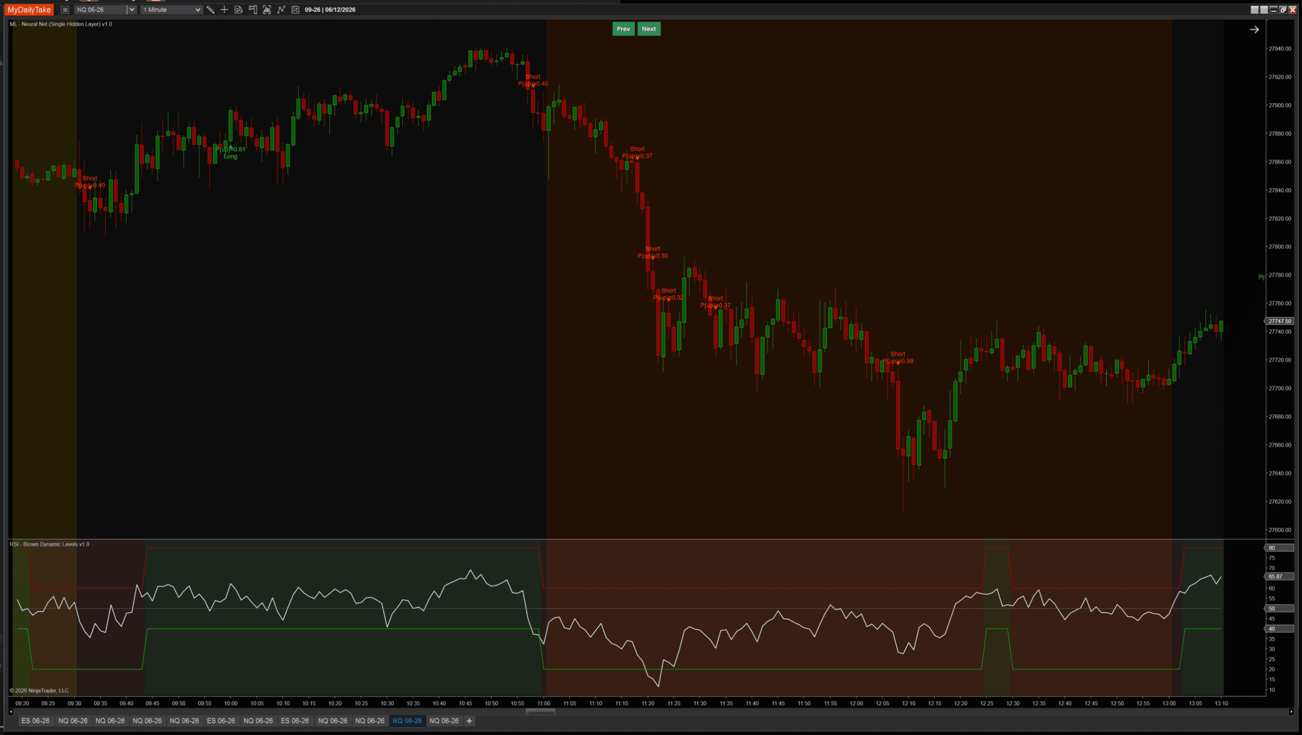
Same defensive pattern as the prior post, for the same reason: the model can produce contrarian signals during sustained trends, and a simple regime filter vetoes them cheaply. RSI(14) above/below 50 is the simplest version — take longs only when RSI confirms uptrend, take shorts only when it confirms downtrend. Below: a clean run with the regime filter active during a sustained downtrend, the network producing aligned shorts as price walks down a stair-step pattern:
Below: the same sustained uptrend, no regime filter on either side, compared by LabelMode. With FavorableExcursion (left), the hidden-layer model still fires contrarian shorts at extreme distFromMa readings — the data’s mean-reversion tendency leaks through even with extra capacity. With CloseToClose (right), the bias is much smaller (consistent with the prior post’s analysis), but it isn’t gone:
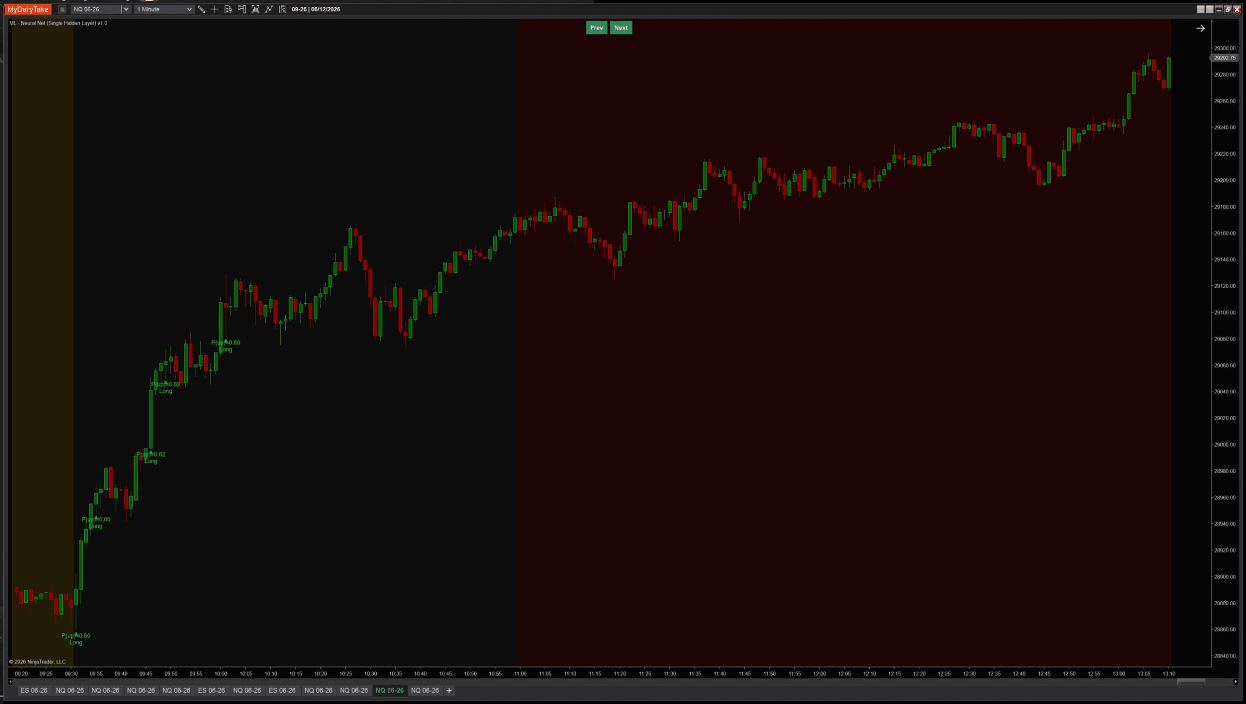
FavorableExcursion labeling — a few contrarian shorts at extremes.
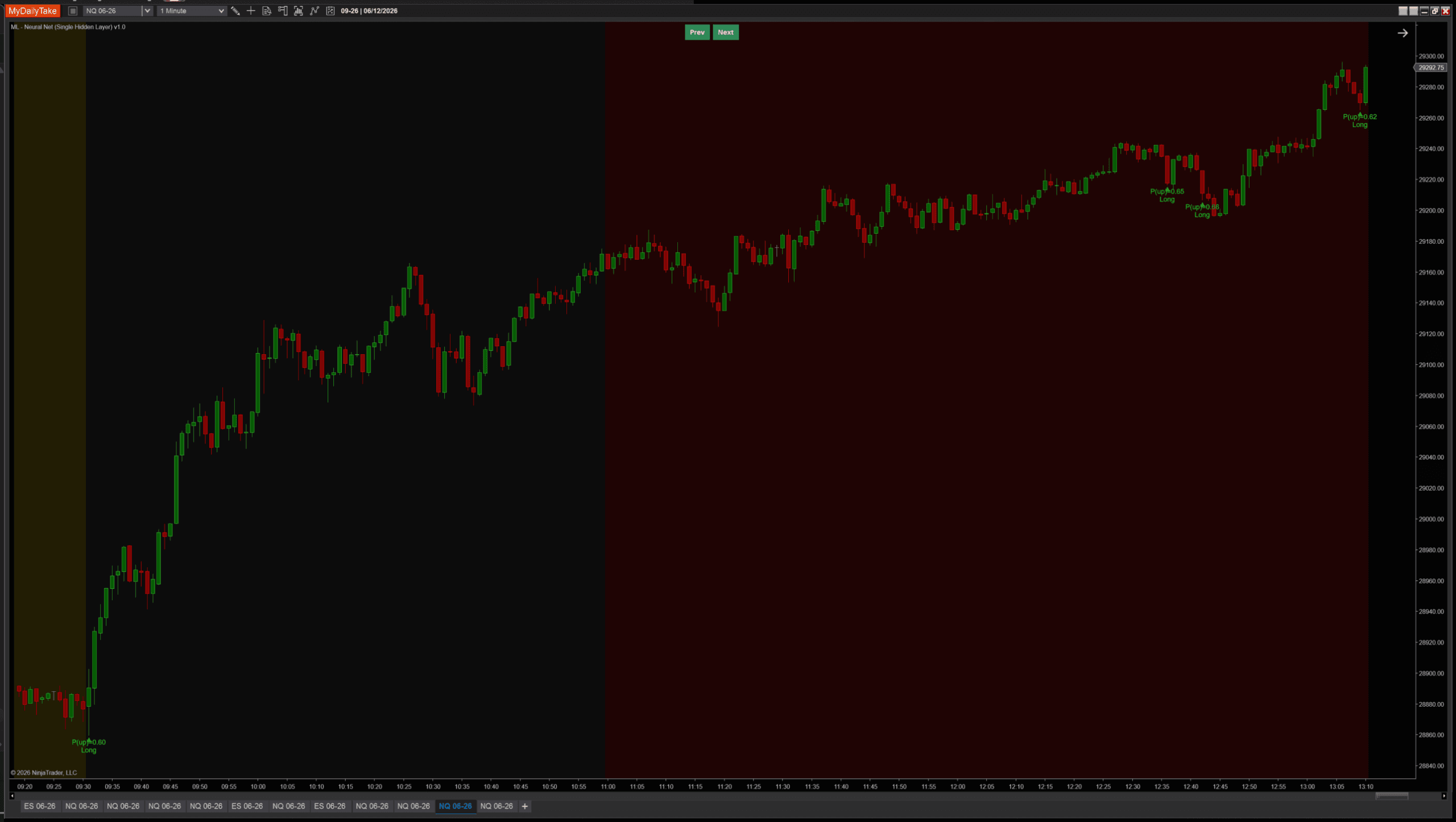
CloseToClose labeling on the same chart — cleaner trend behavior.
🛠️ Using It in a Strategy
Everything the indicator computes is exposed as public Series so any strategy can chain off it directly without recomputing the model. P(up), confidence, and the boolean signal series are all available:
Public Outputs
| Output | Type | Purpose |
|---|---|---|
| ProbabilityUpSeries |
Series | The model's predicted probability of an up move, post-sigmoid output layer. Range [0, 1]. |
| ConfidenceSeries |
Series | |P(up) − 0.5| × 2 — distance from coin-flip, scaled to [0, 1]. 0 = uncertain, 1 = maximum conviction. |
| IsLongSignalSeries |
Series | True on bars where prediction passes the probability gate AND cooldown — long signal fires. |
| IsShortSignalSeries |
Series | True on bars where prediction passes the probability gate AND cooldown — short signal fires. |
Below: a working strategy that combines the network’s signal with an RSI regime filter — long only when the model fires AND RSI confirms uptrend, short only when both confirm downtrend. Same pattern as the prior post’s strategy example, with the neural-net Series plugged in:
private MlNeuralNetSingleHidden     nn;
private RSI                         rsi;

protected override void OnStateChange()
{
    if (State == State.SetDefaults)
    {
        Name        = "ShlRsiTrendFollower";
        Calculate   = Calculate.OnBarClose;
    }
    else if (State == State.DataLoaded)
    {
        nn = MlNeuralNetSingleHidden(
            hiddenNeurons:          6,
            hiddenActivation:       MlNeuralNetSingleHidden_Activation.Tanh,
            randomSeed:             42,
            learningRate:           0.01,
            regularizationLambda:   0.0001,
            labelHorizon:           2,
            weightInit:             MlNeuralNetSingleHidden_WeightInitMode.Random,
            labelMode:              MlNeuralNetSingleHidden_LabelMode.CloseToClose,
            minFavorableMoveAtrs:   1.0,
            maPeriod:               8,
            atrPeriod:              50,
            slopeLookback:          2,
            normalizeFeatures:      true,
            normalizationLookback:  200,
            minProbabilityEdge:     0.10,
            signalCooldownBars:     3);

        rsi = RSI(14, 3);
    }
}

protected override void OnBarUpdate()
{
    if (CurrentBar < 300) return;

    // Long: model predicts up AND RSI confirms uptrend regime.
    if (nn.IsLongSignalSeries[0] && rsi[0] > 50)
        EnterLong("NN Long");

    // Short: model predicts down AND RSI confirms downtrend regime.
    if (nn.IsShortSignalSeries[0] && rsi[0] < 50)
        EnterShort("NN Short");
}
Swap RSI for any indicator that exposes a Series — ADX above a threshold, price relative to a higher-timeframe MA, a SuperTrend state. Anything you already trust as a regime tool will compose cleanly.
📝 The Honest Validation Talk (Still)
Same caveat from the prior post applies here: every prediction is technically out-of-sample (the training step is one LabelHorizon in arrears), but the model is also continuously changing. An “accuracy over the last 1000 bars” figure averages over many different effective models. The number you compute is more a regime-weighted aggregate than a stable model property.
If anything, the situation is sharper for a hidden-layer network. With 31 parameters instead of 4, the model adapts faster to recent regime — meaning even fewer bars in the past actually reflect the model’s current behavior. Walk-forward across multiple regimes is the only honest evaluation, and the work scales with how seriously you want to trust the result.
📦 Download
Install:
- Download the .zip file above.
- In NinjaTrader 8, go to Tools → Import → NinjaScript Add-On.
- Select the downloaded .zip file.
- The indicator will appear under Indicators → indMyDailyTake → ML — Single-Hidden-Layer Neural Net v1.0 on your chart.
🎉 Prop Trading Discounts
💥89% off at Bulenox.com with the code MDT89
This is the third installment of the Learn NinjaScript ML series. Post 1 covered k-Nearest Neighbors, the memorizing model. Post 2 covered online logistic regression, the simplest compressing model. Post 3 (this one) added a hidden layer — the structural step that makes the model a “real” neural network and unlocks the non-linear feature interactions a single neuron can’t represent.